In mathematics, a linear equation is an equation that may be put in the form where are the variables, and are the coefficients, which are often real numbers. The coefficients may be considered as parameters of the equation and may be arbitrary expressions, provided they do not contain any of the variables. To yield a meaningful equation, the coefficients are required to not all be zero.

Cost accounting is defined by the Institute of Management Accountants as "a systematic set of procedures for recording and reporting measurements of the cost of manufacturing goods and performing services in the aggregate and in detail. It includes methods for recognizing, allocating, aggregating and reporting such costs and comparing them with standard costs". Often considered a subset of managerial accounting, its end goal is to advise the management on how to optimize business practices and processes based on cost efficiency and capability. Cost accounting provides the detailed cost information that management needs to control current operations and plan for the future.

In probability theory, a probability density function (PDF), density function, or density of an absolutely continuous random variable, is a function whose value at any given sample in the sample space can be interpreted as providing a relative likelihood that the value of the random variable would be equal to that sample. Probability density is the probability per unit length, in other words, while the absolute likelihood for a continuous random variable to take on any particular value is 0, the value of the PDF at two different samples can be used to infer, in any particular draw of the random variable, how much more likely it is that the random variable would be close to one sample compared to the other sample.
Channel capacity, in electrical engineering, computer science, and information theory, is the theoretical maximum rate at which information can be reliably transmitted over a communication channel.
In probability theory, coupling is a proof technique that allows one to compare two unrelated random variables (distributions) X and Y by creating a random vector W whose marginal distributions correspond to X and Y respectively. The choice of W is generally not unique, and the whole idea of "coupling" is about making such a choice so that X and Y can be related in a particularly desirable way.
In economics, an ordinal utility function is a function representing the preferences of an agent on an ordinal scale. Ordinal utility theory claims that it is only meaningful to ask which option is better than the other, but it is meaningless to ask how much better it is or how good it is. All of the theory of consumer decision-making under conditions of certainty can be, and typically is, expressed in terms of ordinal utility.
In mathematics and economics, the arc elasticity is the elasticity of one variable with respect to another between two given points. It is the ratio of the percentage change of one of the variables between the two points to the percentage change of the other variable. It contrasts with the point elasticity, which is the limit of the arc elasticity as the distance between the two points approaches zero and which hence is defined at a single point rather than for a pair of points.

Contribution margin (CM), or dollar contribution per unit, is the selling price per unit minus the variable cost per unit. "Contribution" represents the portion of sales revenue that is not consumed by variable costs and so contributes to the coverage of fixed costs. This concept is one of the key building blocks of break-even analysis.
In statistics and signal processing, a minimum mean square error (MMSE) estimator is an estimation method which minimizes the mean square error (MSE), which is a common measure of estimator quality, of the fitted values of a dependent variable. In the Bayesian setting, the term MMSE more specifically refers to estimation with quadratic loss function. In such case, the MMSE estimator is given by the posterior mean of the parameter to be estimated. Since the posterior mean is cumbersome to calculate, the form of the MMSE estimator is usually constrained to be within a certain class of functions. Linear MMSE estimators are a popular choice since they are easy to use, easy to calculate, and very versatile. It has given rise to many popular estimators such as the Wiener–Kolmogorov filter and Kalman filter.

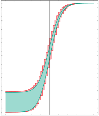
Interval arithmetic is a mathematical technique used to mitigate rounding and measurement errors in mathematical computation by computing function bounds. Numerical methods involving interval arithmetic can guarantee relatively reliable and mathematically correct results. Instead of representing a value as a single number, interval arithmetic or interval mathematics represents each value as a range of possibilities.
In statistics, Poisson regression is a generalized linear model form of regression analysis used to model count data and contingency tables. Poisson regression assumes the response variable Y has a Poisson distribution, and assumes the logarithm of its expected value can be modeled by a linear combination of unknown parameters. A Poisson regression model is sometimes known as a log-linear model, especially when used to model contingency tables.
In geometry, the Hessian curve is a plane curve similar to folium of Descartes. It is named after the German mathematician Otto Hesse. This curve was suggested for application in elliptic curve cryptography, because arithmetic in this curve representation is faster and needs less memory than arithmetic in standard Weierstrass form.
In the design of experiments and analysis of variance, a main effect is the effect of an independent variable on a dependent variable averaged across the levels of any other independent variables. The term is frequently used in the context of factorial designs and regression models to distinguish main effects from interaction effects.
In statistics and econometrics, the multivariate probit model is a generalization of the probit model used to estimate several correlated binary outcomes jointly. For example, if it is believed that the decisions of sending at least one child to public school and that of voting in favor of a school budget are correlated, then the multivariate probit model would be appropriate for jointly predicting these two choices on an individual-specific basis. J.R. Ashford and R.R. Sowden initially proposed an approach for multivariate probit analysis. Siddhartha Chib and Edward Greenberg extended this idea and also proposed simulation-based inference methods for the multivariate probit model which simplified and generalized parameter estimation.
In statistics, pooled variance is a method for estimating variance of several different populations when the mean of each population may be different, but one may assume that the variance of each population is the same. The numerical estimate resulting from the use of this method is also called the pooled variance.
In computer graphics, a digital differential analyzer (DDA) is hardware or software used for interpolation of variables over an interval between start and end point. DDAs are used for rasterization of lines, triangles and polygons. They can be extended to non linear functions, such as perspective correct texture mapping, quadratic curves, and traversing voxels.
In statistics, the antithetic variates method is a variance reduction technique used in Monte Carlo methods. Considering that the error in the simulated signal has a one-over square root convergence, a very large number of sample paths is required to obtain an accurate result. The antithetic variates method reduces the variance of the simulation results.
Hydraulic jump in a rectangular channel, also known as classical jump, is a natural phenomenon that occurs whenever flow changes from supercritical to subcritical flow. In this transition, the water surface rises abruptly, surface rollers are formed, intense mixing occurs, air is entrained, and often a large amount of energy is dissipated. Numeric models created using the standard step method or HEC-RAS are used to track supercritical and subcritical flows to determine where in a specific reach a hydraulic jump will form.
Central place foraging (CPF) theory is an evolutionary ecology model for analyzing how an organism can maximize foraging rates while traveling through a patch, but maintains the key distinction of a forager traveling from a home base to a distant foraging location rather than simply passing through an area or travelling at random. CPF was initially developed to explain how red-winged blackbirds might maximize energy returns when traveling to and from a nest. The model has been further refined and used by anthropologists studying human behavioral ecology and archaeology.
The profit model is the linear, deterministic algebraic model used implicitly by most cost accountants. Starting with, profit equals sales minus costs, it provides a structure for modeling cost elements such as materials, losses, multi-products, learning, depreciation etc. It provides a mutable conceptual base for spreadsheet modelers. This enables them to run deterministic simulations or 'what if' modelling to see the impact of price, cost or quantity changes on profitability.


