Related Research Articles

Statistical inference is the process of using data analysis to infer properties of an underlying distribution of probability. Inferential statistical analysis infers properties of a population, for example by testing hypotheses and deriving estimates. It is assumed that the observed data set is sampled from a larger population.
The likelihood function is the joint probability of observed data viewed as a function of the parameters of a statistical model.

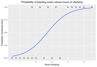
In statistics, the logistic model is a statistical model that models the log-odds of an event as a linear combination of one or more independent variables. In regression analysis, logistic regression is estimating the parameters of a logistic model. Formally, in binary logistic regression there is a single binary dependent variable, coded by an indicator variable, where the two values are labeled "0" and "1", while the independent variables can each be a binary variable or a continuous variable. The corresponding probability of the value labeled "1" can vary between 0 and 1, hence the labeling; the function that converts log-odds to probability is the logistic function, hence the name. The unit of measurement for the log-odds scale is called a logit, from logistic unit, hence the alternative names. See § Background and § Definition for formal mathematics, and § Example for a worked example.

In statistics, an expectation–maximization (EM) algorithm is an iterative method to find (local) maximum likelihood or maximum a posteriori (MAP) estimates of parameters in statistical models, where the model depends on unobserved latent variables. The EM iteration alternates between performing an expectation (E) step, which creates a function for the expectation of the log-likelihood evaluated using the current estimate for the parameters, and a maximization (M) step, which computes parameters maximizing the expected log-likelihood found on the E step. These parameter-estimates are then used to determine the distribution of the latent variables in the next E step. It can be used, for example, to estimate a mixture of gaussians, or to solve the multiple linear regression problem.
The Akaike information criterion (AIC) is an estimator of prediction error and thereby relative quality of statistical models for a given set of data. Given a collection of models for the data, AIC estimates the quality of each model, relative to each of the other models. Thus, AIC provides a means for model selection.
In statistics, a generalized linear model (GLM) is a flexible generalization of ordinary linear regression. The GLM generalizes linear regression by allowing the linear model to be related to the response variable via a link function and by allowing the magnitude of the variance of each measurement to be a function of its predicted value.

In statistics, the coefficient of determination, denoted R2 or r2 and pronounced "R squared", is the proportion of the variation in the dependent variable that is predictable from the independent variable(s).

Regression dilution, also known as regression attenuation, is the biasing of the linear regression slope towards zero, caused by errors in the independent variable.
In statistics, Poisson regression is a generalized linear model form of regression analysis used to model count data and contingency tables. Poisson regression assumes the response variable Y has a Poisson distribution, and assumes the logarithm of its expected value can be modeled by a linear combination of unknown parameters. A Poisson regression model is sometimes known as a log-linear model, especially when used to model contingency tables.

In statistics and numerical analysis, isotonic regression or monotonic regression is the technique of fitting a free-form line to a sequence of observations such that the fitted line is non-decreasing everywhere, and lies as close to the observations as possible.
In statistics, a generalized additive model (GAM) is a generalized linear model in which the linear response variable depends linearly on unknown smooth functions of some predictor variables, and interest focuses on inference about these smooth functions.
In statistics, multinomial logistic regression is a classification method that generalizes logistic regression to multiclass problems, i.e. with more than two possible discrete outcomes. That is, it is a model that is used to predict the probabilities of the different possible outcomes of a categorically distributed dependent variable, given a set of independent variables.
Omnibus tests are a kind of statistical test. They test whether the explained variance in a set of data is significantly greater than the unexplained variance, overall. One example is the F-test in the analysis of variance. There can be legitimate significant effects within a model even if the omnibus test is not significant. For instance, in a model with two independent variables, if only one variable exerts a significant effect on the dependent variable and the other does not, then the omnibus test may be non-significant. This fact does not affect the conclusions that may be drawn from the one significant variable. In order to test effects within an omnibus test, researchers often use contrasts.
In statistics, a generalized estimating equation (GEE) is used to estimate the parameters of a generalized linear model with a possible unmeasured correlation between observations from different timepoints. Although some believe that Generalized estimating equations are robust in everything even with the wrong choice of working-correlation matrix, Generalized estimating equations are only robust to loss of consistency with the wrong choice.
In statistics a quasi-maximum likelihood estimate (QMLE), also known as a pseudo-likelihood estimate or a composite likelihood estimate, is an estimate of a parameter θ in a statistical model that is formed by maximizing a function that is related to the logarithm of the likelihood function, but in discussing the consistency and (asymptotic) variance-covariance matrix, we assume some parts of the distribution may be mis-specified. In contrast, the maximum likelihood estimate maximizes the actual log likelihood function for the data and model. The function that is maximized to form a QMLE is often a simplified form of the actual log likelihood function. A common way to form such a simplified function is to use the log-likelihood function of a misspecified model that treats certain data values as being independent, even when in actuality they may not be. This removes any parameters from the model that are used to characterize these dependencies. Doing this only makes sense if the dependency structure is a nuisance parameter with respect to the goals of the analysis. As long as the quasi-likelihood function that is maximized is not oversimplified, the QMLE is consistent and asymptotically normal. It is less efficient than the maximum likelihood estimate, but may only be slightly less efficient if the quasi-likelihood is constructed so as to minimize the loss of information relative to the actual likelihood. Standard approaches to statistical inference that are used with maximum likelihood estimates, such as the formation of confidence intervals, and statistics for model comparison, can be generalized to the quasi-maximum likelihood setting.
In probability theory and statistics, empirical likelihood (EL) is a nonparametric method for estimating the parameters of statistical models. It requires fewer assumptions about the error distribution while retaining some of the merits in likelihood-based inference. The estimation method requires that the data are independent and identically distributed (iid). It performs well even when the distribution is asymmetric or censored. EL methods can also handle constraints and prior information on parameters. Art Owen pioneered work in this area with his 1988 paper.
Conditional logistic regression is an extension of logistic regression that allows one to account for stratification and matching. Its main field of application is observational studies and in particular epidemiology. It was devised in 1978 by Norman Breslow, Nicholas Day, Katherine Halvorsen, Ross L. Prentice and C. Sabai. It is the most flexible and general procedure for matched data.
David Firth is a British statistician. He is Emeritus Professor in the Department of Statistics at the University of Warwick.
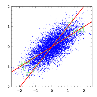
In statistics, linear regression is a statistical model which estimates the linear relationship between a scalar response and one or more explanatory variables. The case of one explanatory variable is called simple linear regression; for more than one, the process is called multiple linear regression. This term is distinct from multivariate linear regression, where multiple correlated dependent variables are predicted, rather than a single scalar variable. If the explanatory variables are measured with error then errors-in-variables models are required, also known as measurement error models.
References
- ↑ Zeng, Guoping; Zeng, Emily (2019). "On the Relationship between Multicollinearity and Separation in Logistic Regression". Communications in Statistics . Simulation and Computation. 50 (7): 1989–1997. doi:10.1080/03610918.2019.1589511. S2CID 132047558.
- ↑ Albert, A.; Anderson, J. A. (1984). "On the Existence of Maximum Likelihood Estimates in Logistic Regression Models". Biometrika. 71 (1–10): 1–10. doi:10.1093/biomet/71.1.1.
- ↑ McCullough, B. D.; Vinod, H. D. (2003). "Verifying the Solution from a Nonlinear Solver: A Case Study". American Economic Review . 93 (3): 873–892. doi:10.1257/000282803322157133. JSTOR 3132121.
- ↑ Cole, S.R.; Chu, H.; Greenland, S. (2014), "Maximum likelihood, profile likelihood, and penalized likelihood: A primer", American Journal of Epidemiology, 179 (2): 252–260, doi: 10.1093/aje/kwt245 , PMC 3873110 , PMID 24173548
- ↑ Sweeting, M.J.; Sutton, A.J.; Lambert, P.C. (2004), "What to add to nothing? Use and avoidance of continuity corrections in meta-analysis of sparse data", Statistics in Medicine, 23 (9): 1351–1375, doi:10.1002/sim.1761, PMID 15116347, S2CID 247667708
- ↑ Mansournia, Mohammad Ali; Geroldinger, Angelika; Greenland, Sander; Heinze, Georg (2018). "Separation in Logistic Regression: Causes, Consequences, and Control". American Journal of Epidemiology . 187 (4): 864–870. doi: 10.1093/aje/kwx299 . PMID 29020135.
- ↑ Gelman, A.; Jakulin, A.; Pittau, M.G.; Su, Y. (2008), "A weakly informative default prior distribution dor logistic and other regression models", Annals of Applied Statistics, 2 (4): 1360–1383, arXiv: 0901.4011 , doi: 10.1214/08-AOAS191