In computational mathematics, an iterative method is a mathematical procedure that uses an initial value to generate a sequence of improving approximate solutions for a class of problems, in which the n-th approximation is derived from the previous ones. A specific implementation of an iterative method, including the termination criteria, is an algorithm of the iterative method. An iterative method is called convergent if the corresponding sequence converges for given initial approximations. A mathematically rigorous convergence analysis of an iterative method is usually performed; however, heuristic-based iterative methods are also common.

In mathematics and physics, Laplace's equation is a second-order partial differential equation named after Pierre-Simon Laplace, who first studied its properties. This is often written as

In physics, the Navier–Stokes equations are certain partial differential equations which describe the motion of viscous fluid substances, named after French engineer and physicist Claude-Louis Navier and Anglo-Irish physicist and mathematician George Gabriel Stokes. They were developed over several decades of progressively building the theories, from 1822 (Navier) to 1842–1850 (Stokes).

The Schrödinger equation is a linear partial differential equation that governs the wave function of a quantum-mechanical system. It is a key result in quantum mechanics, and its discovery was a significant landmark in the development of the subject. The equation is named after Erwin Schrödinger, who postulated the equation in 1925, and published it in 1926, forming the basis for the work that resulted in his Nobel Prize in Physics in 1933.

In mathematics and physics, the heat equation is a certain partial differential equation. Solutions of the heat equation are sometimes known as caloric functions. The theory of the heat equation was first developed by Joseph Fourier in 1822 for the purpose of modeling how a quantity such as heat diffuses through a given region.
The calculus of variations is a field of mathematical analysis that uses variations, which are small changes in functions and functionals, to find maxima and minima of functionals: mappings from a set of functions to the real numbers. Functionals are often expressed as definite integrals involving functions and their derivatives. Functions that maximize or minimize functionals may be found using the Euler–Lagrange equation of the calculus of variations.

Numerical methods for ordinary differential equations are methods used to find numerical approximations to the solutions of ordinary differential equations (ODEs). Their use is also known as "numerical integration", although this term can also refer to the computation of integrals.

In mathematics, a Green's function is the impulse response of an inhomogeneous linear differential operator defined on a domain with specified initial conditions or boundary conditions.
Pseudo-spectral methods, also known as discrete variable representation (DVR) methods, are a class of numerical methods used in applied mathematics and scientific computing for the solution of partial differential equations. They are closely related to spectral methods, but complement the basis by an additional pseudo-spectral basis, which allows representation of functions on a quadrature grid. This simplifies the evaluation of certain operators, and can considerably speed up the calculation when using fast algorithms such as the fast Fourier transform.
In mathematics and its applications, classical Sturm–Liouville theory is the theory of real second-order linear ordinary differential equations of the form:
In mathematics, a Dirichlet problem is the problem of finding a function which solves a specified partial differential equation (PDE) in the interior of a given region that takes prescribed values on the boundary of the region.
The Ritz method is a direct method to find an approximate solution for boundary value problems. The method is named after Walther Ritz, although also commonly called the Rayleigh–Ritz method and the Ritz-Galerkin method.
In mathematics, a change of variables is a basic technique used to simplify problems in which the original variables are replaced with functions of other variables. The intent is that when expressed in new variables, the problem may become simpler, or equivalent to a better understood problem.

In mathematics, delay differential equations (DDEs) are a type of differential equation in which the derivative of the unknown function at a certain time is given in terms of the values of the function at previous times. DDEs are also called time-delay systems, systems with aftereffect or dead-time, hereditary systems, equations with deviating argument, or differential-difference equations. They belong to the class of systems with the functional state, i.e. partial differential equations (PDEs) which are infinite dimensional, as opposed to ordinary differential equations (ODEs) having a finite dimensional state vector. Four points may give a possible explanation of the popularity of DDEs:
- Aftereffect is an applied problem: it is well known that, together with the increasing expectations of dynamic performances, engineers need their models to behave more like the real process. Many processes include aftereffect phenomena in their inner dynamics. In addition, actuators, sensors, and communication networks that are now involved in feedback control loops introduce such delays. Finally, besides actual delays, time lags are frequently used to simplify very high order models. Then, the interest for DDEs keeps on growing in all scientific areas and, especially, in control engineering.
- Delay systems are still resistant to many classical controllers: one could think that the simplest approach would consist in replacing them by some finite-dimensional approximations. Unfortunately, ignoring effects which are adequately represented by DDEs is not a general alternative: in the best situation, it leads to the same degree of complexity in the control design. In worst cases, it is potentially disastrous in terms of stability and oscillations.
- Voluntary introduction of delays can benefit the control system.
- In spite of their complexity, DDEs often appear as simple infinite-dimensional models in the very complex area of partial differential equations (PDEs).
In physics and fluid mechanics, a Blasius boundary layer describes the steady two-dimensional laminar boundary layer that forms on a semi-infinite plate which is held parallel to a constant unidirectional flow. Falkner and Skan later generalized Blasius' solution to wedge flow, i.e. flows in which the plate is not parallel to the flow.
The Poisson–Boltzmann equation is a useful equation in many settings, whether it be to understand physiological interfaces, polymer science, electron interactions in a semiconductor, or more. It aims to describe the distribution of the electric potential in solution in the direction normal to a charged surface. This distribution is important to determine how the electrostatic interactions will affect the molecules in solution. The Poisson–Boltzmann equation is derived via mean-field assumptions. From the Poisson–Boltzmann equation many other equations have been derived with a number of different assumptions.
In mathematics and numerical analysis, an adaptive step size is used in some methods for the numerical solution of ordinary differential equations in order to control the errors of the method and to ensure stability properties such as A-stability. Using an adaptive stepsize is of particular importance when there is a large variation in the size of the derivative. For example, when modeling the motion of a satellite about the earth as a standard Kepler orbit, a fixed time-stepping method such as the Euler method may be sufficient. However things are more difficult if one wishes to model the motion of a spacecraft taking into account both the Earth and the Moon as in the Three-body problem. There, scenarios emerge where one can take large time steps when the spacecraft is far from the Earth and Moon, but if the spacecraft gets close to colliding with one of the planetary bodies, then small time steps are needed. Romberg's method and Runge–Kutta–Fehlberg are examples of a numerical integration methods which use an adaptive stepsize.
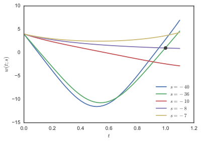
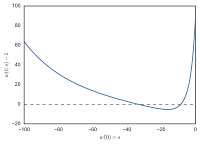
In the area of mathematics known as numerical ordinary differential equations, the direct multiple shooting method is a numerical method for the solution of boundary value problems. The method divides the interval over which a solution is sought into several smaller intervals, solves an initial value problem in each of the smaller intervals, and imposes additional matching conditions to form a solution on the whole interval. The method constitutes a significant improvement in distribution of nonlinearity and numerical stability over single shooting methods.
In the science of fluid flow, Stokes' paradox is the phenomenon that there can be no creeping flow of a fluid around a disk in two dimensions; or, equivalently, the fact there is no non-trivial steady-state solution for the Stokes equations around an infinitely long cylinder. This is opposed to the 3-dimensional case, where Stokes' method provides a solution to the problem of flow around a sphere.
In combustion, Frank-Kamenetskii theory explains the thermal explosion of a homogeneous mixture of reactants, kept inside a closed vessel with constant temperature walls. It is named after a Russian scientist David A. Frank-Kamenetskii, who along with Nikolay Semenov developed the theory in the 1930s.