The Navier–Stokes equations are partial differential equations which describe the motion of viscous fluid substances, named after French engineer and physicist Claude-Louis Navier and Irish physicist and mathematician George Gabriel Stokes. They were developed over several decades of progressively building the theories, from 1822 (Navier) to 1842–1850 (Stokes).

The electrical resistance of an object is a measure of its opposition to the flow of electric current. Its reciprocal quantity is electrical conductance, measuring the ease with which an electric current passes. Electrical resistance shares some conceptual parallels with mechanical friction. The SI unit of electrical resistance is the ohm, while electrical conductance is measured in siemens (S).
Electrical resistivity is a fundamental specific property of a material that measures its electrical resistance or how strongly it resists electric current. A low resistivity indicates a material that readily allows electric current. Resistivity is commonly represented by the Greek letter ρ (rho). The SI unit of electrical resistivity is the ohm-metre (Ω⋅m). For example, if a 1 m3 solid cube of material has sheet contacts on two opposite faces, and the resistance between these contacts is 1 Ω, then the resistivity of the material is 1 Ω⋅m.

In physics, Gauss's law, also known as Gauss's flux theorem, is a law relating the distribution of electric charge to the resulting electric field. In its integral form, it states that the flux of the electric field out of an arbitrary closed surface is proportional to the electric charge enclosed by the surface, irrespective of how that charge is distributed. Even though the law alone is insufficient to determine the electric field across a surface enclosing any charge distribution, this may be possible in cases where symmetry mandates uniformity of the field. Where no such symmetry exists, Gauss's law can be used in its differential form, which states that the divergence of the electric field is proportional to the local density of charge.
In fluid dynamics, Stokes' law is an empirical law for the frictional force – also called drag force – exerted on spherical objects with very small Reynolds numbers in a viscous fluid. It was derived by George Gabriel Stokes in 1851 by solving the Stokes flow limit for small Reynolds numbers of the Navier–Stokes equations.
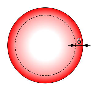
In electromagnetism, skin effect is the tendency of an alternating electric current (AC) to become distributed within a conductor such that the current density is largest near the surface of the conductor and decreases exponentially with greater depths in the conductor. It is caused by opposing eddy currents induced by the changing magnetic field resulting from the alternating current. The electric current flows mainly at the "skin" of the conductor, between the outer surface and a level called the skin depth. Skin depth depends on the frequency of the alternating current; as frequency increases, current flow becomes more concentrated near the surface, resulting in less skin depth. Skin effect reduces the effective cross-section of the conductor and thus increases its effective resistance. At 60 Hz in copper, skin depth is about 8.5 mm. At high frequencies skin depth becomes much smaller.
The van der Pauw Method is a technique commonly used to measure the resistivity and the Hall coefficient of a sample. Its power lies in its ability to accurately measure the properties of a sample of any arbitrary shape, as long as the sample is approximately two-dimensional, solid, and the electrodes are placed on its perimeter. The van der Pauw method employs a four-point probe placed around the perimeter of the sample, in contrast to the linear four point probe: this allows the van der Pauw method to provide an average resistivity of the sample, whereas a linear array provides the resistivity in the sensing direction. This difference becomes important for anisotropic materials, which can be properly measured using the Montgomery Method, an extension of the van der Pauw Method.
Joule heating is the process by which the passage of an electric current through a conductor produces heat.
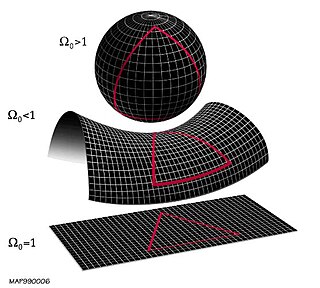
The flatness problem is a cosmological fine-tuning problem within the Big Bang model of the universe. Such problems arise from the observation that some of the initial conditions of the universe appear to be fine-tuned to very 'special' values, and that small deviations from these values would have extreme effects on the appearance of the universe at the current time.

Sheet resistance, is the resistance of a square piece of a thin material with contacts made to two opposite sides of the square. It is usually a measurement of electrical resistance of thin films that are uniform in thickness. It is commonly used to characterize materials made by semiconductor doping, metal deposition, resistive paste printing, and glass coating. Examples of these processes are: doped semiconductor regions, and the resistors that are screen printed onto the substrates of thick-film hybrid microcircuits.
The Transfer Length Method or the "Transmission Line Model" is a technique used in semiconductor physics and engineering to determine the specific contact resistivity between a metal and a semiconductor. TLM has been developed because with the ongoing device shrinkage in microelectronics the relative contribution of the contact resistance at metal-semiconductor interfaces in a device could not be neglected any more and an accurate measurement method for determining the specific contact resistivity was required.

Electrical resistivity tomography (ERT) or electrical resistivity imaging (ERI) is a geophysical technique for imaging sub-surface structures from electrical resistivity measurements made at the surface, or by electrodes in one or more boreholes. If the electrodes are suspended in the boreholes, deeper sections can be investigated. It is closely related to the medical imaging technique electrical impedance tomography (EIT), and mathematically is the same inverse problem. In contrast to medical EIT, however, ERT is essentially a direct current method. A related geophysical method, induced polarization, measures the transient response and aims to determine the subsurface chargeability properties.

In electrical engineering, earth potential rise (EPR), also called ground potential rise (GPR), occurs when a large current flows to earth through an earth grid impedance. The potential relative to a distant point on the Earth is highest at the point where current enters the ground, and declines with distance from the source. Ground potential rise is a concern in the design of electrical substations because the high potential may be a hazard to people or equipment.

An electrode array is a configuration of electrodes used for measuring either an electric current or voltage. Some electrode arrays can operate in a bidirectional fashion, in that they can also be used to provide a stimulating pattern of electric current or voltage.
Spontaneous potentials are often measured down boreholes for formation evaluation in the oil and gas industry, and they can also be measured along the Earth's surface for mineral exploration or groundwater investigation. The phenomenon and its application to geology was first recognized by Conrad Schlumberger, Marcel Schlumberger, and E.G. Leonardon in 1931, and the first published examples were from Romanian oil fields.
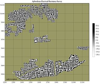
Electrical resistance surveys are one of a number of methods used in archaeological geophysics, as well as in engineering geological investigations. In this type of survey electrical resistance meters are used to detect and map subsurface archaeological features and patterning.

Electro Thermal Dynamic Stripping Process (ET-DSP) is a patented in situ thermal environmental remediation technology, created by McMillan-McGee Corporation, for cleaning contaminated sites. ET-DSP uses readily available three phase electric power to heat the subsurface with electrodes. Electrodes are placed at various depths and locations in the formation. Electric current to each electrode is controlled continuously by computer to uniformly heat the target contamination zone.
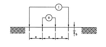
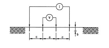
Concrete electrical resistivity can be obtained by applying a current into the concrete and measuring the response voltage. There are different methods for measuring concrete resistivity.
Vertical electrical sounding (VES) is a geophysical method for investigation of a geological medium. The method is based on the estimation of the electrical conductivity or resistivity of the medium. The estimation is performed based on the measurement of voltage of electrical field induced by the distant grounded electrodes.
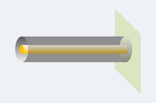
Space cloth is a hypothetical infinite plane of conductive material having a resistance of η ohms per square, where η is the impedance of free space. η ≈ 376.7 ohms. If a transmission line composed of straight parallel perfect conductors in free space is terminated by space cloth that is normal to the transmission line then that transmission line is terminated by its characteristic impedance. The calculation of the characteristic impedance of a transmission line composed of straight, parallel good conductors may be replaced by the calculation of the D.C. resistance between electrodes placed on a two-dimensional resistive surface. This equivalence can be used in reverse to calculate the resistance between two conductors on a resistive sheet if the arrangement of the conductors is the same as the cross section of a transmission line of known impedance. For example, a pad surrounded by a guard ring on a printed circuit board (PCB) is similar to the cross section of a coaxial cable transmission line.