Spatial join

Last updated January 13, 2023

A spatial join is an operation in a geographic information system (GIS) or spatial database that combines the attribute tables of two spatial layers based on a desired spatial relation between their geometries.^[1] It is similar to the table join operation in relational databases in merging two tables, but each pair of rows is correlated based on some form of matching location rather than a common key value.^[2] It is also similar to vector overlay operations common in GIS software such as Intersect and Union in merging two spatial datasets, but the output does not contain a composite geometry, only merged attributes.

Spatial joins are used in a variety of spatial analysis and management applications, including allocating individuals to districts and statistical aggregation. Spatial join is found in most, if not all, GIS and spatial database software, although this term is not always used, and sometimes it must be derived indirectly by the combination of several tools.

Spatial relation predicates

Examples of topological spatial relations. TopologicSpatialRelarions2.png — Examples of topological spatial relations.

Fundamental to the spatial join operation is the formulation of a spatial relationship between two geometric primitives as a logical predicate; that is, a criterion that can be evaluated as true or false.^[3] For example, "A is less than 5km from B" would be true if the distance between points A and B is 3km, and false if the distance is 10km. These relation predicates can be of two types:

A Topological relation is a qualitative relationship between two shapes that does not depend on a measurable space (that is, coordinates). Common examples of such predicates include "A is completely inside B," "A overlaps B," "A is adjacent to B" (i.e., sharing a boundary but no interior), and "A is disjoint from B" (not touching at all). These are commonly specified according to some form of the 9-Intersection Model,^[4] which is incorporated into the international Simple Feature Access specification (ISO 19125-2).^[5]
A Metric relation is a quantitative (measurable) relationship between two shapes in a coordinate space, most commonly a distance or direction. Common examples include "A is due north of B" or "A is less than 5 km from B." Not all software implementations support metric relations.

Note that some relations are commutative (e.g., A overlaps B if and only if B overlaps A) while others are not (e.g., A is within B does not mean B is within A).

The geometric primitives involved in these relations may be of any dimension (points, lines, or regions), but some relations may only have meaning with certain dimensions. For example, "A is within B" has a clear meaning if A is a point and B is a region, but is meaningless if both A and B are points. Other relations may be vague; for example, the distance between two regions or two lines may be interpreted as the minimal distance between their closest boundaries, or a mean distance between their centroids.^[6]

Operation

As in a relational table join as defined in the relational algebra, two input layers or tables are provided (hereafter X and Y), and the output is a table containing all of the columns of each of the inputs (or some subset thereof if selected by the user). The rows of the new table are a subset of Cross join or Cartesian product of the two tables, all possible pairs of rows {X1-Y1, X1-Y2, X1-Y3, X2-Y1, X2-Y2, X2-Y3, X3-Y1, X3-Y2, X3-Y3, ...}. Rather than include all possible combinations, each pair is evaluated according to the given spatial predicate; those for which the predicate is true are considered "matching" and are retained, while those for which the predicate is false are discarded.

For example, consider the following two tables:

Students table
StudentID	LastName	GPA	Residence: point
1	Rafferty	3.56	•
2	Jones	2.75	•
3	Heisenberg	3.98	•
4	Robinson	1.56	•
5	Smith	2.67	•
6	Williams	3.46	•

Schools table
SchoolID	SchoolName	District: polygon	Building: point
31	Belknap Elementary	□	•
33	Parkview Elementary	□	•
34	Smith Elementary	□	•
35	Central Elementary	□	•

When the spatial join is executed, the direction of attachment must be specified, for two reasons: 1) the given spatial predicate may not be commutative, and 2) there is often a many-to-one relationship between the rows (e.g., many students are inside each school district). In the example above, a common goal would be to join the schools table to the students table (the target table), with the relation predicate being "student.residence within school.district." Assuming that the districts do not overlap, each student point will be in no more than one school district, so the output would have the same rows as the students table, with the corresponding school attributes attached, as:

Students x Schools
StudentID	LastName	GPA	Residence: point	SchoolID	SchoolName
1	Rafferty	3.56	•	33	Parkview Elementary
2	Jones	2.75	•	34	Smith Elementary
3	Heisenberg	3.98	•	35	Central Elementary
4	Robinson	1.56	•	33	Parkview Elementary
5	Smith	2.67	•	34	Smith Elementary
6	Williams	3.46	•	33	Parkview Elementary

The reverse operation, in this case attaching the student information to the schools table, is not as simple because many rows must be joined to one row. Some GIS software does not allow this operation, but most implementations allow for an aggregate join, in which aggregate summaries of the matching rows can be included, such as arrays, counts, sums, or means.^[7] For example, the result table might look like:

Schools x Students
SchoolID	SchoolName	District: polygon	Building: point	Students_COUNT	GPA_MEAN
31	Belknap Elementary	□	•	0	`NULL`
33	Parkview Elementary	□	•	3	2.86
34	Smith Elementary	□	•	2	2.71
35	Central Elementary	□	•	1	3.98

Another option when there are multiple matches is to use some criterion to select one of the rows from the matching set, usually a spatial optimization criterion.^[2]^[8] For example, one could join the school building points (not the districts) to the student residents points by selecting the school that is nearest to each student. Not all software implements this option directly, although in some cases it can be derived through a combination of tools.

External links

Spatial Join tool in ArcGIS Pro
Join attributes by location tool in QGIS
Join attributes by nearest tool in QGIS
Spatial Join in Manifold GIS
Spatial Joins in PostGIS

Related Research Articles

A geographic information system (GIS) is a type of database containing geographic data, combined with software tools for managing, analyzing, and visualizing those data. In a broader sense, one may consider such a system to also include human users and support staff, procedures and workflows, body of knowledge of relevant concepts and methods, and institutional organizations.

In mathematics, a finitary relation over sets X₁, ..., X_n is a subset of the Cartesian product X₁ × ⋯ × X_n; that is, it is a set of n-tuples (x₁, ..., x_n) consisting of elements x_i in X_i. Typically, the relation describes a possible connection between the elements of an n-tuple. For example, the relation "x is divisible by y and z" consists of the set of 3-tuples such that when substituted to x, y and z, respectively, make the sentence true.

A relational database is a database based on the relational model of data, as proposed by E. F. Codd in 1970. A system used to maintain relational databases is a relational database management system (RDBMS). Many relational database systems are equipped with the option of using the SQL for querying and maintaining the database.

The relational model (RM) is an approach to managing data using a structure and language consistent with first-order predicate logic, first described in 1969 by English computer scientist Edgar F. Codd, where all data is represented in terms of tuples, grouped into relations. A database organized in terms of the relational model is a relational database.

In database theory, relational algebra is a theory that uses algebraic structures with a well-founded semantics for modeling data, and defining queries on it. The theory was introduced by Edgar F. Codd.

A GIS file format is a standard for encoding geographical information into a computer file, as a specialized type of file format for use in geographic information systems (GIS) and other geospatial applications. Since the 1970s, dozens of formats have been created based on various data models for various purposes. They have been created by government mapping agencies, GIS software vendors, standards bodies such as the Open Geospatial Consortium, informal user communities, and even individual developers.

A join clause in SQL – corresponding to a join operation in relational algebra – combines columns from one or more tables into a new table. Informally, a join stitches two tables and puts on the same row records with matching fields : INNER, LEFT OUTER, RIGHT OUTER, FULL OUTER and CROSS.

A GIS software program is a computer program to support the use of a geographic information system, providing the ability to create, store, manage, query, analyze, and visualize geographic data, that is, data representing phenomena for which location is important. The GIS software industry encompasses a broad range of commercial and open-source products that provide some or all of these capabilities within various information technology architectures.

VMDS abbreviates the relational database technology called Version Managed Data Store provided by GE Energy as part of its Smallworld technology platform and was designed from the outset to store and analyse the highly complex spatial and topological networks typically used by enterprise utilities such as power distribution and telecommunications.

A spatial database is a general-purpose database that has been enhanced to include spatial data that represents objects defined in a geometric space, along with tools for querying and analyzing such data. Most spatial databases allow the representation of simple geometric objects such as points, lines and polygons. Some spatial databases handle more complex structures such as 3D objects, topological coverages, linear networks, and triangulated irregular networks (TINs). While typical databases have developed to manage various numeric and character types of data, such databases require additional functionality to process spatial data types efficiently, and developers have often added geometry or feature data types. The Open Geospatial Consortium (OGC) developed the Simple Features specification and sets standards for adding spatial functionality to database systems. The SQL/MM Spatial ISO/IEC standard is a part the SQL/MM multimedia standard and extends the Simple Features standard with data types that support circular interpolations. Almost all current relational and object-relational database management systems now have spatial extensions, and some GIS software vendors have developed their own spatial extensions to database management systems.

QGIS is a free and open-source cross-platform desktop geographic information system (GIS) application that supports viewing, editing, printing, and analysis of geospatial data.

Georeferencing or georegistration is a type of coordinate transformation that binds a digital raster image or vector database that represents a geographic space to a spatial reference system, thus locating the digital data in the real world. It is thus the geographic form of image registration. The term can refer to the mathematical formulas used to perform the transformation, the metadata stored alongside or within the image file to specify the transformation, or the process of manually or automatically aligning the image to the real world to create such metadata. The most common result is that the image can be visually and analytically integrated with other geographic data in geographic information systems and remote sensing software.

A georelational data model is a geographic data model that represents geographic features as an interrelated set of spatial and attribute data. The georelational model was the dominant form of vector file format during the 1980s and 1990s, including the Esri coverage and Shapefile.

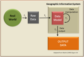
A geographic data model, geospatial data model, or simply data model in the context of geographic information systems, is a mathematical and digital structure for representing phenomena over the Earth. Generally, such data models represent various aspects of these phenomena by means of geographic data, including spatial locations, attributes, change over time, and identity. For example, the vector data model represents geography as collections of points, lines, and polygons, and the raster data model represent geography as cell matrices that store numeric values. Data models are implemented throughout the GIS ecosystem, including the software tools for data management and spatial analysis, data stored in a variety of GIS file formats, specifications and standards, and specific designs for GIS installations.

In database theory, a relation, as originally defined by E. F. Codd, is a set of tuples (d₁, d₂, ..., d_n), where each element d_j is a member of D_j, a data domain. Codd's original definition notwithstanding, and contrary to the usual definition in mathematics, there is no ordering to the elements of the tuples of a relation. Instead, each element is termed an attribute value. An attribute is a name paired with a domain. An attribute value is an attribute name paired with an element of that attribute's domain, and a tuple is a set of attribute values in which no two distinct elements have the same name. Thus, in some accounts, a tuple is described as a function, mapping names to values.

Proximity analysis is a class of spatial analysis tools and algorithms that employ geographic distance as a central principle. Distance is fundamental to geographic inquiry and spatial analysis, due to principles such as the friction of distance, Tobler's first law of geography, and Spatial autocorrelation, which are incorporated into analytical tools. Proximity methods are thus used in a variety of applications, especially those that involve movement and interaction.

<span class="mw-page-title-main">DE-9IM</span>

The Dimensionally Extended 9-Intersection Model (DE-9IM) is a topological model and a standard used to describe the spatial relations of two regions, in geometry, point-set topology, geospatial topology, and fields related to computer spatial analysis. The spatial relations expressed by the model are invariant to rotation, translation and scaling transformations.

<span class="mw-page-title-main">Geospatial topology</span> Type of spatial relationship

Geospatial topology is the study and application of qualitative spatial relationships between geographic features, or between representations of such features in geographic information, such as in geographic information systems (GIS). For example, the fact that two regions overlap or that one contains the other are examples of topological relationships. It is thus the application of the mathematics of topology to GIS, and is distinct from, but complementary to the many aspects of geographic information that are based on quantitative spatial measurements through coordinate geometry. Topology appears in many aspects of geographic information science and GIS practice, including the discovery of inherent relationships through spatial query, vector overlay and map algebra; the enforcement of expected relationships as validation rules stored in geospatial data; and the use of stored topological relationships in applications such as network analysis. Spatial topology is the generalization of geospatial topology for non-geographic domains, e.g., CAD software.

Vector overlay is an operation in a geographic information system (GIS) for integrating two or more vector spatial data sets. Terms such as polygon overlay, map overlay, and topological overlay are often used synonymously, although they are not identical in the range of operations they include. Overlay has been one of the core elements of spatial analysis in GIS since its early development. Some overlay operations, especially Intersect and Union, are implemented in all GIS software and are used in a wide variety of analytical applications, while others are less common.

A Geodatabase is a type of GIS file format for representing spatial data in a geographic information system. It is both a logical data model developed by Esri in the late 1990s, a GIS software vendor, and the physical implementation of that logical model in several proprietary file formats released during the 2000s. The geodatabase design is based on the spatial database model for storing spatial data in relational and object-relational databases. Given the dominance of Esri in the GIS industry, the term "geodatabase" is used by some as a generic trademark for any spatial database, regardless of platform or design.

References

↑ Longley, Paul A.; Goodchild, Michael F.; Maguire, David J.; Rhind, David W. (2011). Geographic Information Systems & Science (3rd ed.). Wiley. p. 360.
1 2 Campbell, Jonathan; Shin, Michael (2011). Essentials of Geographic Information Systems. Saylor Foundation. p. 182. ISBN 9781453321966 . Retrieved 5 January 2023.
↑ "Join attributes by location tool". QGIS 3.22 Documentation. OSGeo. Retrieved 4 January 2023.
↑ Egenhofer, M.J.; Herring, J.R. (1990). "A Mathematical Framework for the Definition of Topological Relationships" (PDF). Archived from the original (PDF) on 2010-06-14.{{cite journal}}: Cite journal requires |journal= (help)
↑ Open Geospatial Consortium. "Simple Feature Access - Part 2: SQL Option". Open Geospatial Consortium Standards. Retrieved 4 January 2023.
↑ Worboys, Michael; Duckham, Matt (2004). GIS: A Computing Perspective (2nd ed.). Boca Raton, Florida: CRC Press. p. 195. ISBN 0-415-28375-2.
↑ "Spatial Join (Analysis)". ArcGIS Pro Documentation. Esri. Retrieved 5 January 2023.
↑ "Join attributes by nearest tool". QGIS 3.22 Documentation. OSGeo. Retrieved 4 January 2023.

This page is based on this Wikipedia article
Text is available under the CC BY-SA 4.0 license; additional terms may apply.
Images, videos and audio are available under their respective licenses.

[Longley2011-1] Longley, Paul A.; Goodchild, Michael F.; Maguire, David J.; Rhind, David W. (2011). Geographic Information Systems & Science (3rd ed.). Wiley. p. 360.

[campbell2011-2] 1 2 Campbell, Jonathan; Shin, Michael (2011). Essentials of Geographic Information Systems. Saylor Foundation. p. 182. ISBN 9781453321966 . Retrieved 5 January 2023.

[qgis-3] "Join attributes by location tool". QGIS 3.22 Documentation. OSGeo. Retrieved 4 January 2023.

[sdh1990-4] Egenhofer, M.J.; Herring, J.R. (1990). "A Mathematical Framework for the Definition of Topological Relationships" (PDF). Archived from the original (PDF) on 2010-06-14.{{cite journal}}: Cite journal requires |journal= (help)

[OGC-SFA-5] Open Geospatial Consortium. "Simple Feature Access - Part 2: SQL Option". Open Geospatial Consortium Standards. Retrieved 4 January 2023.

[worboys2004-6] Worboys, Michael; Duckham, Matt (2004). GIS: A Computing Perspective (2nd ed.). Boca Raton, Florida: CRC Press. p. 195. ISBN 0-415-28375-2.

[7] "Spatial Join (Analysis)". ArcGIS Pro Documentation. Esri. Retrieved 5 January 2023.

[qgis-nearest-8] "Join attributes by nearest tool". QGIS 3.22 Documentation. OSGeo. Retrieved 4 January 2023.

[1]

[2]

[3]

[4]

[5]

[6]

[7]

[8]