
In theoretical physics, quantum field theory (QFT) is a theoretical framework that combines classical field theory, special relativity, and quantum mechanics. QFT is used in particle physics to construct physical models of subatomic particles and in condensed matter physics to construct models of quasiparticles.
In fluid dynamics, turbulence or turbulent flow is fluid motion characterized by chaotic changes in pressure and flow velocity. It is in contrast to a laminar flow, which occurs when a fluid flows in parallel layers, with no disruption between those layers.
In physics, a Langevin equation is a stochastic differential equation describing how a system evolves when subjected to a combination of deterministic and fluctuating ("random") forces. The dependent variables in a Langevin equation typically are collective (macroscopic) variables changing only slowly in comparison to the other (microscopic) variables of the system. The fast (microscopic) variables are responsible for the stochastic nature of the Langevin equation. One application is to Brownian motion, which models the fluctuating motion of a small particle in a fluid.
In fluid dynamics, the Darcy–Weisbach equation is an empirical equation that relates the head loss, or pressure loss, due to friction along a given length of pipe to the average velocity of the fluid flow for an incompressible fluid. The equation is named after Henry Darcy and Julius Weisbach. Currently, there is no formula more accurate or universally applicable than the Darcy-Weisbach supplemented by the Moody diagram or Colebrook equation.
In mathematics, the Hodge star operator or Hodge star is a linear map defined on the exterior algebra of a finite-dimensional oriented vector space endowed with a nondegenerate symmetric bilinear form. Applying the operator to an element of the algebra produces the Hodge dual of the element. This map was introduced by W. V. D. Hodge.
In fluid dynamics, Kolmogorov microscales are the smallest scales in the turbulent flow of fluids. At the Kolmogorov scale, viscosity dominates and the turbulence kinetic energy is dissipated into heat. They are defined by
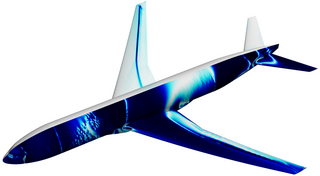
In fluid dynamics, turbulence modeling is the construction and use of a mathematical model to predict the effects of turbulence. Turbulent flows are commonplace in most real-life scenarios, including the flow of blood through the cardiovascular system, the airflow over an aircraft wing, the re-entry of space vehicles, besides others. In spite of decades of research, there is no analytical theory to predict the evolution of these turbulent flows. The equations governing turbulent flows can only be solved directly for simple cases of flow. For most real-life turbulent flows, CFD simulations use turbulent models to predict the evolution of turbulence. These turbulence models are simplified constitutive equations that predict the statistical evolution of turbulent flows.
A direct numerical simulation (DNS) is a simulation in computational fluid dynamics (CFD) in which the Navier–Stokes equations are numerically solved without any turbulence model. This means that the whole range of spatial and temporal scales of the turbulence must be resolved. All the spatial scales of the turbulence must be resolved in the computational mesh, from the smallest dissipative scales, up to the integral scale , associated with the motions containing most of the kinetic energy. The Kolmogorov scale, , is given by
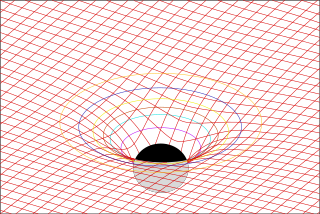
In physics, Maxwell's equations in curved spacetime govern the dynamics of the electromagnetic field in curved spacetime or where one uses an arbitrary coordinate system. These equations can be viewed as a generalization of the vacuum Maxwell's equations which are normally formulated in the local coordinates of flat spacetime. But because general relativity dictates that the presence of electromagnetic fields induce curvature in spacetime, Maxwell's equations in flat spacetime should be viewed as a convenient approximation.
In fluid dynamics, turbulence kinetic energy (TKE) is the mean kinetic energy per unit mass associated with eddies in turbulent flow. Physically, the turbulence kinetic energy is characterised by measured root-mean-square (RMS) velocity fluctuations. In the Reynolds-averaged Navier Stokes equations, the turbulence kinetic energy can be calculated based on the closure method, i.e. a turbulence model.
The plasma parameter is a dimensionless number, denoted by capital Lambda, Λ. The plasma parameter is usually interpreted to be the argument of the Coulomb logarithm, which is the ratio of the maximum impact parameter to the classical distance of closest approach in Coulomb scattering. In this case, the plasma parameter is given by:
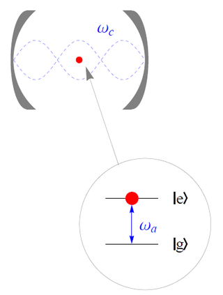
The Jaynes–Cummings model is a theoretical model in quantum optics. It describes the system of a two-level atom interacting with a quantized mode of an optical cavity, with or without the presence of light. It was originally developed to study the interaction of atoms with the quantized electromagnetic field in order to investigate the phenomena of spontaneous emission and absorption of photons in a cavity.
The time-evolving block decimation (TEBD) algorithm is a numerical scheme used to simulate one-dimensional quantum many-body systems, characterized by at most nearest-neighbour interactions. It is dubbed Time-evolving Block Decimation because it dynamically identifies the relevant low-dimensional Hilbert subspaces of an exponentially larger original Hilbert space. The algorithm, based on the Matrix Product States formalism, is highly efficient when the amount of entanglement in the system is limited, a requirement fulfilled by a large class of quantum many-body systems in one dimension.

In fluid dynamics, eddy diffusion, eddy dispersion, or turbulent diffusion is a process by which fluid substances mix together due to eddy motion. These eddies can vary widely in size, from subtropical ocean gyres down to the small Kolmogorov microscales, and occur as a result of turbulence. The theory of eddy diffusion was first developed by Sir Geoffrey Ingram Taylor.

In fluid mechanics, the Reynolds number is a dimensionless quantity that helps predict fluid flow patterns in different situations by measuring the ratio between inertial and viscous forces. At low Reynolds numbers, flows tend to be dominated by laminar (sheet-like) flow, while at high Reynolds numbers, flows tend to be turbulent. The turbulence results from differences in the fluid's speed and direction, which may sometimes intersect or even move counter to the overall direction of the flow. These eddy currents begin to churn the flow, using up energy in the process, which for liquids increases the chances of cavitation.
In fluid and molecular dynamics, the Batchelor scale, determined by George Batchelor (1959), describes the size of a droplet of fluid that will diffuse in the same time it takes the energy in an eddy of size η to dissipate. The Batchelor scale can be determined by:
In quantum field theory, and especially in quantum electrodynamics, the interacting theory leads to infinite quantities that have to be absorbed in a renormalization procedure, in order to be able to predict measurable quantities. The renormalization scheme can depend on the type of particles that are being considered. For particles that can travel asymptotically large distances, or for low energy processes, the on-shell scheme, also known as the physical scheme, is appropriate. If these conditions are not fulfilled, one can turn to other schemes, like the minimal subtraction scheme.
The spin angular momentum of light (SAM) is the component of angular momentum of light that is associated with the quantum spin and the rotation between the polarization degrees of freedom of the photon.
Lagrangian field theory is a formalism in classical field theory. It is the field-theoretic analogue of Lagrangian mechanics. Lagrangian mechanics is used to analyze the motion of a system of discrete particles each with a finite number of degrees of freedom. Lagrangian field theory applies to continua and fields, which have an infinite number of degrees of freedom.
The two-dimensional critical Ising model is the critical limit of the Ising model in two dimensions. It is a two-dimensional conformal field theory whose symmetry algebra is the Virasoro algebra with the central charge . Correlation functions of the spin and energy operators are described by the minimal model. While the minimal model has been exactly solved, see also, e.g., the article on Ising critical exponents, the solution does not cover other observables such as connectivities of clusters.


