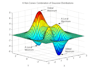
A likelihood function measures how well a statistical model explains observed data by calculating the probability of seeing that data under different parameter values of the model. It is constructed from the joint probability distribution of the random variable that (presumably) generated the observations. When evaluated on the actual data points, it becomes a function solely of the model parameters.
Bayesian inference is a method of statistical inference in which Bayes' theorem is used to calculate a probability of a hypothesis, given prior evidence, and update it as more information becomes available. Fundamentally, Bayesian inference uses a prior distribution to estimate posterior probabilities. Bayesian inference is an important technique in statistics, and especially in mathematical statistics. Bayesian updating is particularly important in the dynamic analysis of a sequence of data. Bayesian inference has found application in a wide range of activities, including science, engineering, philosophy, medicine, sport, and law. In the philosophy of decision theory, Bayesian inference is closely related to subjective probability, often called "Bayesian probability".
In statistics, maximum likelihood estimation (MLE) is a method of estimating the parameters of an assumed probability distribution, given some observed data. This is achieved by maximizing a likelihood function so that, under the assumed statistical model, the observed data is most probable. The point in the parameter space that maximizes the likelihood function is called the maximum likelihood estimate. The logic of maximum likelihood is both intuitive and flexible, and as such the method has become a dominant means of statistical inference.
A Bayesian network is a probabilistic graphical model that represents a set of variables and their conditional dependencies via a directed acyclic graph (DAG). While it is one of several forms of causal notation, causal networks are special cases of Bayesian networks. Bayesian networks are ideal for taking an event that occurred and predicting the likelihood that any one of several possible known causes was the contributing factor. For example, a Bayesian network could represent the probabilistic relationships between diseases and symptoms. Given symptoms, the network can be used to compute the probabilities of the presence of various diseases.
In probability theory and statistics, a Gaussian process is a stochastic process, such that every finite collection of those random variables has a multivariate normal distribution. The distribution of a Gaussian process is the joint distribution of all those random variables, and as such, it is a distribution over functions with a continuous domain, e.g. time or space.
The posterior probability is a type of conditional probability that results from updating the prior probability with information summarized by the likelihood via an application of Bayes' rule. From an epistemological perspective, the posterior probability contains everything there is to know about an uncertain proposition, given prior knowledge and a mathematical model describing the observations available at a particular time. After the arrival of new information, the current posterior probability may serve as the prior in another round of Bayesian updating.
In mathematical statistics, the Fisher information is a way of measuring the amount of information that an observable random variable X carries about an unknown parameter θ of a distribution that models X. Formally, it is the variance of the score, or the expected value of the observed information.
A marginal likelihood is a likelihood function that has been integrated over the parameter space. In Bayesian statistics, it represents the probability of generating the observed sample for all possible values of the parameters; it can be understood as the probability of the model itself and is therefore often referred to as model evidence or simply evidence.
In statistical decision theory, an admissible decision rule is a rule for making a decision such that there is no other rule that is always "better" than it, in the precise sense of "better" defined below. This concept is analogous to Pareto efficiency.
In Bayesian statistics, a maximum a posteriori probability (MAP) estimate is an estimate of an unknown quantity, that equals the mode of the posterior distribution. The MAP can be used to obtain a point estimate of an unobserved quantity on the basis of empirical data. It is closely related to the method of maximum likelihood (ML) estimation, but employs an augmented optimization objective which incorporates a prior distribution over the quantity one wants to estimate. MAP estimation can therefore be seen as a regularization of maximum likelihood estimation.
In statistics, M-estimators are a broad class of extremum estimators for which the objective function is a sample average. Both non-linear least squares and maximum likelihood estimation are special cases of M-estimators. The definition of M-estimators was motivated by robust statistics, which contributed new types of M-estimators. However, M-estimators are not inherently robust, as is clear from the fact that they include maximum likelihood estimators, which are in general not robust. The statistical procedure of evaluating an M-estimator on a data set is called M-estimation. The "M" initial stands for "maximum likelihood-type".
Bootstrapping is a procedure for estimating the distribution of an estimator by resampling one's data or a model estimated from the data. Bootstrapping assigns measures of accuracy to sample estimates. This technique allows estimation of the sampling distribution of almost any statistic using random sampling methods.
In Bayesian inference, the Bernstein–von Mises theorem provides the basis for using Bayesian credible sets for confidence statements in parametric models. It states that under some conditions, a posterior distribution converges in total variation distance to a multivariate normal distribution centered at the maximum likelihood estimator with covariance matrix given by , where is the true population parameter and is the Fisher information matrix at the true population parameter value:
In probability theory and statistics, the Dirichlet process (DP) is one of the most popular Bayesian nonparametric models. It was introduced by Thomas Ferguson as a prior over probability distributions.
In statistical decision theory, a randomised decision rule or mixed decision rule is a decision rule that associates probabilities with deterministic decision rules. In finite decision problems, randomised decision rules define a risk set which is the convex hull of the risk points of the nonrandomised decision rules.
In statistics, when selecting a statistical model for given data, the relative likelihood compares the relative plausibilities of different candidate models or of different values of a parameter of a single model.
In variational Bayesian methods, the evidence lower bound is a useful lower bound on the log-likelihood of some observed data.

Stochastic gradient Langevin dynamics (SGLD) is an optimization and sampling technique composed of characteristics from Stochastic gradient descent, a Robbins–Monro optimization algorithm, and Langevin dynamics, a mathematical extension of molecular dynamics models. Like stochastic gradient descent, SGLD is an iterative optimization algorithm which uses minibatching to create a stochastic gradient estimator, as used in SGD to optimize a differentiable objective function. Unlike traditional SGD, SGLD can be used for Bayesian learning as a sampling method. SGLD may be viewed as Langevin dynamics applied to posterior distributions, but the key difference is that the likelihood gradient terms are minibatched, like in SGD. SGLD, like Langevin dynamics, produces samples from a posterior distribution of parameters based on available data. First described by Welling and Teh in 2011, the method has applications in many contexts which require optimization, and is most notably applied in machine learning problems.

In machine learning, a variational autoencoder (VAE) is an artificial neural network architecture introduced by Diederik P. Kingma and Max Welling. It is part of the families of probabilistic graphical models and variational Bayesian methods.
A Stein discrepancy is a statistical divergence between two probability measures that is rooted in Stein's method. It was first formulated as a tool to assess the quality of Markov chain Monte Carlo samplers, but has since been used in diverse settings in statistics, machine learning and computer science.


