The method of least squares is a parameter estimation method in regression analysis based on minimizing the sum of the squares of the residuals made in the results of each individual equation.
A hidden Markov model (HMM) is a Markov model in which the observations are dependent on a latent Markov process. An HMM requires that there be an observable process whose outcomes depend on the outcomes of in a known way. Since cannot be observed directly, the goal is to learn about state of by observing By definition of being a Markov model, an HMM has an additional requirement that the outcome of at time must be "influenced" exclusively by the outcome of at and that the outcomes of and at must be conditionally independent of at given at time Estimation of the parameters in an HMM can be performed using maximum likelihood. For linear chain HMMs, the Baum–Welch algorithm can be used to estimate the parameters.
Pattern recognition is the task of assigning a class to an observation based on patterns extracted from data. While similar, pattern recognition (PR) is not to be confused with pattern machines (PM) which may possess (PR) capabilities but their primary function is to distinguish and create emergent patterns. PR has applications in statistical data analysis, signal processing, image analysis, information retrieval, bioinformatics, data compression, computer graphics and machine learning. Pattern recognition has its origins in statistics and engineering; some modern approaches to pattern recognition include the use of machine learning, due to the increased availability of big data and a new abundance of processing power.

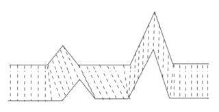
In time series analysis, dynamic time warping (DTW) is an algorithm for measuring similarity between two temporal sequences, which may vary in speed. For instance, similarities in walking could be detected using DTW, even if one person was walking faster than the other, or if there were accelerations and decelerations during the course of an observation. DTW has been applied to temporal sequences of video, audio, and graphics data — indeed, any data that can be turned into a one-dimensional sequence can be analyzed with DTW. A well-known application has been automatic speech recognition, to cope with different speaking speeds. Other applications include speaker recognition and online signature recognition. It can also be used in partial shape matching applications.

In statistics, an expectation–maximization (EM) algorithm is an iterative method to find (local) maximum likelihood or maximum a posteriori (MAP) estimates of parameters in statistical models, where the model depends on unobserved latent variables. The EM iteration alternates between performing an expectation (E) step, which creates a function for the expectation of the log-likelihood evaluated using the current estimate for the parameters, and a maximization (M) step, which computes parameters maximizing the expected log-likelihood found on the E step. These parameter-estimates are then used to determine the distribution of the latent variables in the next E step. It can be used, for example, to estimate a mixture of gaussians, or to solve the multiple linear regression problem.

In digital image processing and computer vision, image segmentation is the process of partitioning a digital image into multiple image segments, also known as image regions or image objects. The goal of segmentation is to simplify and/or change the representation of an image into something that is more meaningful and easier to analyze. Image segmentation is typically used to locate objects and boundaries in images. More precisely, image segmentation is the process of assigning a label to every pixel in an image such that pixels with the same label share certain characteristics.
In statistics, Gibbs sampling or a Gibbs sampler is a Markov chain Monte Carlo (MCMC) algorithm for sampling from a specified multivariate probability distribution when direct sampling from the joint distribution is difficult, but sampling from the conditional distribution is more practical. This sequence can be used to approximate the joint distribution ; to approximate the marginal distribution of one of the variables, or some subset of the variables ; or to compute an integral. Typically, some of the variables correspond to observations whose values are known, and hence do not need to be sampled.
In electrical engineering, statistical computing and bioinformatics, the Baum–Welch algorithm is a special case of the expectation–maximization algorithm used to find the unknown parameters of a hidden Markov model (HMM). It makes use of the forward-backward algorithm to compute the statistics for the expectation step.
In statistics, a mixture model is a probabilistic model for representing the presence of subpopulations within an overall population, without requiring that an observed data set should identify the sub-population to which an individual observation belongs. Formally a mixture model corresponds to the mixture distribution that represents the probability distribution of observations in the overall population. However, while problems associated with "mixture distributions" relate to deriving the properties of the overall population from those of the sub-populations, "mixture models" are used to make statistical inferences about the properties of the sub-populations given only observations on the pooled population, without sub-population identity information. Mixture models are used for clustering, under the name model-based clustering, and also for density estimation.
The forward algorithm, in the context of a hidden Markov model (HMM), is used to calculate a 'belief state': the probability of a state at a certain time, given the history of evidence. The process is also known as filtering. The forward algorithm is closely related to, but distinct from, the Viterbi algorithm.

In probability and statistics, the Dirichlet distribution (after Peter Gustav Lejeune Dirichlet), often denoted , is a family of continuous multivariate probability distributions parameterized by a vector of positive reals. It is a multivariate generalization of the beta distribution, hence its alternative name of multivariate beta distribution (MBD). Dirichlet distributions are commonly used as prior distributions in Bayesian statistics, and in fact, the Dirichlet distribution is the conjugate prior of the categorical distribution and multinomial distribution.
A phase-type distribution is a probability distribution constructed by a convolution or mixture of exponential distributions. It results from a system of one or more inter-related Poisson processes occurring in sequence, or phases. The sequence in which each of the phases occurs may itself be a stochastic process. The distribution can be represented by a random variable describing the time until absorption of a Markov process with one absorbing state. Each of the states of the Markov process represents one of the phases.
Conditional random fields (CRFs) are a class of statistical modeling methods often applied in pattern recognition and machine learning and used for structured prediction. Whereas a classifier predicts a label for a single sample without considering "neighbouring" samples, a CRF can take context into account. To do so, the predictions are modelled as a graphical model, which represents the presence of dependencies between the predictions. What kind of graph is used depends on the application. For example, in natural language processing, "linear chain" CRFs are popular, for which each prediction is dependent only on its immediate neighbours. In image processing, the graph typically connects locations to nearby and/or similar locations to enforce that they receive similar predictions.
In probability theory and statistics, a categorical distribution is a discrete probability distribution that describes the possible results of a random variable that can take on one of K possible categories, with the probability of each category separately specified. There is no innate underlying ordering of these outcomes, but numerical labels are often attached for convenience in describing the distribution,. The K-dimensional categorical distribution is the most general distribution over a K-way event; any other discrete distribution over a size-K sample space is a special case. The parameters specifying the probabilities of each possible outcome are constrained only by the fact that each must be in the range 0 to 1, and all must sum to 1.
The discrete phase-type distribution is a probability distribution that results from a system of one or more inter-related geometric distributions occurring in sequence, or phases. The sequence in which each of the phases occur may itself be a stochastic process. The distribution can be represented by a random variable describing the time until absorption of an absorbing Markov chain with one absorbing state. Each of the states of the Markov chain represents one of the phases.
Structured prediction or structured (output) learning is an umbrella term for supervised machine learning techniques that involves predicting structured objects, rather than scalar discrete or real values.
In statistics, a maximum-entropy Markov model (MEMM), or conditional Markov model (CMM), is a graphical model for sequence labeling that combines features of hidden Markov models (HMMs) and maximum entropy (MaxEnt) models. An MEMM is a discriminative model that extends a standard maximum entropy classifier by assuming that the unknown values to be learnt are connected in a Markov chain rather than being conditionally independent of each other. MEMMs find applications in natural language processing, specifically in part-of-speech tagging and information extraction.

In statistics and signal processing, step detection is the process of finding abrupt changes in the mean level of a time series or signal. It is usually considered as a special case of the statistical method known as change detection or change point detection. Often, the step is small and the time series is corrupted by some kind of noise, and this makes the problem challenging because the step may be hidden by the noise. Therefore, statistical and/or signal processing algorithms are often required.
In statistics and machine learning, the hierarchical Dirichlet process (HDP) is a nonparametric Bayesian approach to clustering grouped data. It uses a Dirichlet process for each group of data, with the Dirichlet processes for all groups sharing a base distribution which is itself drawn from a Dirichlet process. This method allows groups to share statistical strength via sharing of clusters across groups. The base distribution being drawn from a Dirichlet process is important, because draws from a Dirichlet process are atomic probability measures, and the atoms will appear in all group-level Dirichlet processes. Since each atom corresponds to a cluster, clusters are shared across all groups. It was developed by Yee Whye Teh, Michael I. Jordan, Matthew J. Beal and David Blei and published in the Journal of the American Statistical Association in 2006, as a formalization and generalization of the infinite hidden Markov model published in 2002.
In computer vision, rigid motion segmentation is the process of separating regions, features, or trajectories from a video sequence into coherent subsets of space and time. These subsets correspond to independent rigidly moving objects in the scene. The goal of this segmentation is to differentiate and extract the meaningful rigid motion from the background and analyze it. Image segmentation techniques labels the pixels to be a part of pixels with certain characteristics at a particular time. Here, the pixels are segmented depending on its relative movement over a period of time i.e. the time of the video sequence.


