Step detection

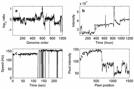
Examples of signals that may contain steps corrupted by noise. (a) DNA copy-number ratios from microarray data, (b) cosmic ray intensity from a neutron monitor, (c) rotation speed against time of R. Sphaeroides flagellar motor, and (d) red pixel intensity from a single scan line of a digital image.

In statistics and signal processing, step detection (also known as step smoothing, step filtering, shift detection, jump detection or edge detection ) is the process of finding abrupt changes (steps, jumps, shifts) in the mean level of a time series or signal. It is usually considered as a special case of the statistical method known as change detection or change point detection. Often, the step is small and the time series is corrupted by some kind of noise, and this makes the problem challenging because the step may be hidden by the noise. Therefore, statistical and/or signal processing algorithms are often required.

The step detection problem occurs in multiple scientific and engineering contexts, for example in statistical process control ^[1] (the control chart being the most directly related method), in exploration geophysics (where the problem is to segment a well-log recording into stratigraphic zones ^[2] ), in genetics (the problem of separating microarray data into similar copy-number regimes ^[3] ), and in biophysics (detecting state transitions in a molecular machine as recorded in time-position traces ^[4] ). For 2D signals, the related problem of edge detection has been studied intensively for image processing. ^[5]

Algorithms

When the step detection must be performed as and when the data arrives, then online algorithms are usually used, ^[6] and it becomes a special case of sequential analysis. Such algorithms include the classical CUSUM method applied to changes in mean. ^[7]

By contrast, offline algorithms are applied to the data potentially long after it has been received. Most offline algorithms for step detection in digital data can be categorised as top-down, bottom-up, sliding window, or global methods.

Top-down

These algorithms start with the assumption that there are no steps and introduce possible candidate steps one at a time, testing each candidate to find the one that minimizes some criteria (such as the least-squares fit of the estimated, underlying piecewise constant signal). An example is the stepwise jump placement algorithm, first studied in geophysical problems, ^[2] that has found recent uses in modern biophysics. ^[8]

Bottom-up

Bottom-up algorithms take the "opposite" approach to top-down methods, first assuming that there is a step in between every sample in the digital signal, and then successively merging steps based on some criteria tested for every candidate merge.

Sliding window

By considering a small "window" of the signal, these algorithms look for evidence of a step occurring within the window. The window "slides" across the time series, one time step at a time. The evidence for a step is tested by statistical procedures, for example, by use of the two-sample Student's t-test. Alternatively, a nonlinear filter such as the median filter is applied to the signal. Filters such as these attempt to remove the noise whilst preserving the abrupt steps.

Global

Global algorithms consider the entire signal in one go, and attempt to find the steps in the signal by some kind of optimization procedure. Algorithms include wavelet methods, ^[9] and total variation denoising which uses methods from convex optimization. Where the steps can be modelled as a Markov chain, then Hidden Markov Models are also often used (a popular approach in the biophysics community ^[10] ). When there are only a few unique values of the mean, then k-means clustering can also be used.

Linear versus nonlinear signal processing methods for step detection

Because steps and (independent) noise have theoretically infinite bandwidth and so overlap in the Fourier basis, signal processing approaches to step detection generally do not use classical smoothing techniques such as the low pass filter. Instead, most algorithms are explicitly nonlinear or time-varying. ^[11]

Step detection and piecewise constant signals

Because the aim of step detection is to find a series of instantaneous jumps in the mean of a signal, the wanted, underlying, mean signal is piecewise constant. For this reason, step detection can be profitably viewed as the problem of recovering a piecewise constant signal corrupted by noise. There are two complementary models for piecewise constant signals: as 0-degree splines with a few knots, or as level sets with a few unique levels. Many algorithms for step detection are therefore best understood as either 0-degree spline fitting, or level set recovery, methods.

Step detection as level set recovery

When there are only a few unique values of the mean, clustering techniques such as k-means clustering or mean-shift are appropriate. These techniques are best understood as methods for finding a level set description of the underlying piecewise constant signal.

Step detection as 0-degree spline fitting

Many algorithms explicitly fit 0-degree splines to the noisy signal in order to detect steps (including stepwise jump placement methods ^{[2] [8]} ), but there are other popular algorithms that can also be seen to be spline fitting methods after some transformation, for example total variation denoising. ^[12]

Generalized step detection by piecewise constant denoising

All the algorithms mentioned above have certain advantages and disadvantages in particular circumstances, yet, a surprisingly large number of these step detection algorithms are special cases of a more general algorithm. ^[11] This algorithm involves the minimization of a global functional: ^[13]

${\displaystyle H[m]=\sum _{i=1}^{N}\sum _{j=1}^{N}\Lambda (x_{i}-m_{j},m_{i}-m_{j},x_{i}-x_{j},i-j)}$

(1)

Here, x_i for i = 1, ...., N is the discrete-time input signal of length N, and m_i is the signal output from the algorithm. The goal is to minimize H[m] with respect to the output signal m. The form of the function ${\displaystyle \scriptstyle \Lambda }$ determines the particular algorithm. For example, choosing:

${\displaystyle \Lambda ={\frac {1}{2}}\left|x_{i}-m_{j}\right|^{2}I(i-j=0)+\gamma \left|m_{i}-m_{j}\right|I(i-j=1)}$

where I(S) = 0 if the condition S is false, and one otherwise, obtains the total variation denoising algorithm with regularization parameter ${\displaystyle \gamma }$. Similarly:

${\displaystyle \Lambda =\min \left\{{\frac {1}{2}}\left|m_{i}-m_{j}\right|^{2},W\right\}}$

leads to the mean shift algorithm, when using an adaptive step size Euler integrator initialized with the input signal x. ^[13] Here W > 0 is a parameter that determines the support of the mean shift kernel. Another example is:

${\displaystyle \Lambda ={\frac {1-\exp(-\beta |m_{i}-m_{j}|^{2}/2)}{\beta }}\cdot I(|i-j|\leq W)}$

leading to the bilateral filter, where ${\displaystyle \scriptstyle \beta >0}$ is the tonal kernel parameter, and W is the spatial kernel support. Yet another special case is:

${\displaystyle \Lambda ={\frac {1}{2}}\left|x_{i}-m_{j}\right|^{2}I(i-j=0)+\gamma \left|m_{i}-m_{j}\right|^{0}I(i-j=1)}$

specifying a group of algorithms that attempt to greedily fit 0-degree splines to the signal. ^{[2] [8]} Here, ${\displaystyle \scriptstyle \left|x\right|^{0}}$ is defined as zero if x = 0, and one otherwise.

Many of the functionals in equation ( 1 ) defined by the particular choice of ${\displaystyle \scriptstyle \Lambda }$ are convex: they can be minimized using methods from convex optimization. Still others are non-convex but a range of algorithms for minimizing these functionals have been devised. ^[13]

Step detection using the Potts model

A classical variational method for step detection is the Potts model. It is given by the non-convex optimization problem

${\displaystyle u^{*}=\arg \min _{u\in \mathbb {R} ^{N}}\gamma \|\nabla u\|_{0}+\|u-x\|_{p}^{p}}$

The term ${\displaystyle \|\nabla u\|_{0}=\#\{i:u_{i}\neq u_{i+1}\}}$ penalizes the number of jumps and the term ${\displaystyle \|u-x\|_{p}^{p}=\sum _{i=1}^{N}|u_{i}-x_{i}|^{p}}$ measures fidelity to data x. The parameter γ > 0 controls the tradeoff between regularity and data fidelity. Since the minimizer ${\displaystyle u^{*}}$ is piecewise constant the steps are given by the non-zero locations of the gradient ${\displaystyle \nabla u^{*}}$. For ${\displaystyle p=2}$ and ${\displaystyle p=1}$ there are fast algorithms which give an exact solution of the Potts problem in ${\displaystyle O(N^{2})}$. ^{[14] [15] [16] [17]}

See also

• Time-series segmentation

References

1. E.S. Page (1955). "A test for a change in a parameter occurring at an unknown point". Biometrika. 42 (3–4): 523–527. doi:10.1093/biomet/42.3-4.523. hdl: 10338.dmlcz/103435 .
2. Gill, D. (1970). "Application of a statistical zonation method to reservoir evaluation and digitized log analysis". American Association of Petroleum Geologists Bulletin. 54: 719–729. doi:10.1306/5d25ca35-16c1-11d7-8645000102c1865d.
3. Snijders, A.M.; et al. (2001). "Assembly of microarrays for genome-wide measurement of DNA copy number". Nature Genetics. 29 (3): 263–264. doi:10.1038/ng754. PMID   11687795. S2CID   19460203.
4. Sowa, Y.; Rowe, A. D.; Leake, M. C.; Yakushi, T.; Homma, M.; Ishijima, A.; Berry, R. M. (2005). "Direct observation of steps in rotation of the bacterial flagellar motor". Nature. 437 (7060): 916–919. Bibcode:2005Natur.437..916S. doi:10.1038/nature04003. PMID   16208378. S2CID   262329024.
5. Serra, J.P. (1982). Image analysis and mathematical morphology. London; New York: Academic Press.
6. Basseville, M.; I.V. Nikiforov (1993). Detection of Abrupt Changes: Theory and Application. Prentice Hall.
7. Rodionov, S.N., 2005a: A brief overview of the regime shift detection methods. link to PDF In: Large-Scale Disturbances (Regime Shifts) and Recovery in Aquatic Ecosystems: Challenges for Management Toward Sustainability, V. Velikova and N. Chipev (Eds.), UNESCO-ROSTE/BAS Workshop on Regime Shifts, 14–16 June 2005, Varna, Bulgaria, 17-24.
8. Kerssemakers, J.W.J.; Munteanu, E.L.; Laan, L.; Noetzel, T.L.; Janson, M.E.; Dogterom, M. (2006). "Assembly dynamics of microtubules at molecular resolution". Nature. 442 (7103): 709–712. Bibcode:2006Natur.442..709K. doi:10.1038/nature04928. PMID   16799566. S2CID   4359681.
9. Mallat, S.; Hwang, W.L. (1992). "Singularity detection and processing with wavelets". IEEE Transactions on Information Theory. 38 (2): 617–643. CiteSeerX   10.1.1.36.5153 . doi:10.1109/18.119727.
10. McKinney, S. A.; Joo, C.; Ha, T. (2006). "Analysis of Single-Molecule FRET Trajectories Using Hidden Markov Modeling". Biophysical Journal. 91 (5): 1941–1951. Bibcode:2006BpJ....91.1941M. doi:10.1529/biophysj.106.082487. PMC   1544307 . PMID   16766620.
11. Little, M.A.; Jones, N.S. (2011). "Generalized methods and solvers for noise removal from piecewise constant signals: Part I. Background theory". Proceedings of the Royal Society A . 467 (2135): 3088–3114. Bibcode:2011RSPSA.467.3088L. doi:10.1098/rspa.2010.0671. PMC   3191861 . PMID   22003312.
12. Chan, D.; T. Chan (2003). "Edge-preserving and scale-dependent properties of total variation regularization". Inverse Problems. 19 (6): S165–S187. Bibcode:2003InvPr..19S.165S. doi:10.1088/0266-5611/19/6/059. S2CID   30704800.
13. Mrazek, P.; Weickert, J.; Bruhn, A. (2006). "On robust estimation and smoothing with spatial and tonal kernels". Geometric properties for incomplete data. Berlin, Germany: Springer.
14. Mumford, D., & Shah, J. (1989). Optimal approximations by piecewise smooth functions and associated variational problems. Communications on pure and applied mathematics, 42(5), 577-685.
15. Winkler, G.; Liebscher, V. (2002). "Smoothers for discontinuous signals". Journal of Nonparametric Statistics. 14 (1–2): 203–222. doi:10.1080/10485250211388. S2CID   119562495.
16. Friedrich; et al. (2008). "Complexity penalized M-estimation: fast computation". Journal of Computational and Graphical Statistics. 17 (1): 201–224. doi:10.1198/106186008x285591. S2CID   117951377.
17. A. Weinmann, M. Storath, L. Demaret. "The ${\displaystyle L^{1}}$-Potts functional for robust jump-sparse reconstruction." SIAM Journal on Numerical Analysis, 53(1):644-673 (2015).

External links

• PWCTools: Flexible Matlab and Python software for step detection by piecewise constant denoising
• Pottslab: Matlab toolbox for piecewise constant estimation based on the Potts model