Related Research Articles
Econometrics is the application of statistical methods to economic data in order to give empirical content to economic relationships. More precisely, it is "the quantitative analysis of actual economic phenomena based on the concurrent development of theory and observation, related by appropriate methods of inference". An introductory economics textbook describes econometrics as allowing economists "to sift through mountains of data to extract simple relationships". The first known use of the term "econometrics" was by Polish economist Paweł Ciompa in 1910. Jan Tinbergen is considered by many to be one of the founding fathers of econometrics. Ragnar Frisch is credited with coining the term in the sense in which it is used today.

In economics, the Gini coefficient, sometimes called the Gini index or Gini ratio, is a measure of statistical dispersion intended to represent the income inequality or wealth inequality within a nation or any other group of people. It was developed by the Italian statistician and sociologist Corrado Gini and published in his 1912 paper Variability and Mutability.
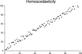
In statistics, a sequence of random variables is homoscedastic if all its random variables have the same finite variance. This is also known as homogeneity of variance. The complementary notion is called heteroscedasticity. The spellings homoskedasticity and heteroskedasticity are also frequently used.
Income inequality metrics or income distribution metrics are used by social scientists to measure the distribution of income and economic inequality among the participants in a particular economy, such as that of a specific country or of the world in general. While different theories may try to explain how income inequality comes about, income inequality metrics simply provide a system of measurement used to determine the dispersion of incomes. The concept of inequality is distinct from poverty and fairness.
The Current Population Survey (CPS) is a monthly survey of about 60,000 U.S. households conducted by the United States Census Bureau for the Bureau of Labor Statistics (BLS). The BLS uses the data to publish reports early each month called the Employment Situation. This report provides estimates of the unemployment rate and the numbers of employed and unemployed people in the United States based on the CPS. A readable Employment Situation Summary is provided monthly. Annual estimates include employment and unemployment in large metropolitan areas. Researchers can use some CPS microdata to investigate these or other topics.

In statistics, a vector of random variables is heteroscedastic if the variability of the random disturbance is different across elements of the vector. Here, variability could be quantified by the variance or any other measure of statistical dispersion. Thus heteroscedasticity is the absence of homoscedasticity. A typical example is the set of observations of income in different cities.

The distribution of wealth is a comparison of the wealth of various members or groups in a society. It shows one aspect of economic inequality or economic heterogeneity.
In statistics, econometrics, epidemiology and related disciplines, the method of instrumental variables (IV) is used to estimate causal relationships when controlled experiments are not feasible or when a treatment is not successfully delivered to every unit in a randomized experiment. Intuitively, IVs are used when an explanatory variable of interest is correlated with the error term, in which case ordinary least squares and ANOVA give biased results. A valid instrument induces changes in the explanatory variable but has no independent effect on the dependent variable, allowing a researcher to uncover the causal effect of the explanatory variable on the dependent variable.

In statistics, ordinary least squares (OLS) is a type of linear least squares method for estimating the unknown parameters in a linear regression model. OLS chooses the parameters of a linear function of a set of explanatory variables by the principle of least squares: minimizing the sum of the squares of the differences between the observed dependent variable in the given dataset and those predicted by the linear function.
In statistics and econometrics, panel data and longitudinal data are both multi-dimensional data involving measurements over time. Panel data is a subset of longitudinal data where observations are for the same subjects each time.
In statistics, a tobit model is any of a class of regression models in which the observed range of the dependent variable is censored in some way. The term was coined by Arthur Goldberger in reference to James Tobin, who developed the model in 1958 to mitigate the problem of zero-inflated data for observations of household expenditure on durable goods. Because Tobin's method can be easily extended to handle truncated and other non-randomly selected samples, some authors adopt a broader definition of the tobit model that includes these cases.
Censored regression models are a class of models in which the dependent variable is censored above or below a certain threshold. A commonly used likelihood-based model to accommodate to a censored sample is the Tobit model, but quantile and nonparametric estimators have also been developed. These and other censored regression models are often confused with truncated regression models. Truncated regression models are used for data where whole observations are missing so that the values for the dependent and the independent variables are unknown. Censored regression models are used for data where only the value for the dependent variable is unknown while the values of the independent variables are still available.

Wealth inequality in the United States, also known as the wealth gap, is the unequal distribution of assets among residents of the United States. Wealth commonly includes the values of any homes, automobiles, personal valuables, businesses, savings, and investments, as well as any associated debts. The net worth of U.S. households and non-profit organizations was $107 trillion in the third quarter of 2019, a record level both in nominal terms and purchasing power parity. As of Q3 2019, the bottom 50% of households had $1.67 trillion, or 1.6% of the net worth, versus $74.5 trillion, or 70% for the top 10%. From an international perspective, the difference in US median and mean wealth per adult is over 600%.
Choice modelling attempts to model the decision process of an individual or segment via revealed preferences or stated preferences made in a particular context or contexts. Typically, it attempts to use discrete choices in order to infer positions of the items on some relevant latent scale. Indeed many alternative models exist in econometrics, marketing, sociometrics and other fields, including utility maximization, optimization applied to consumer theory, and a plethora of other identification strategies which may be more or less accurate depending on the data, sample, hypothesis and the particular decision being modelled. In addition, choice modelling is regarded as the most suitable method for estimating consumers' willingness to pay for quality improvements in multiple dimensions.
The Heckman correction is a statistical technique to correct bias from non-randomly selected samples or otherwise incidentally truncated dependent variables, a pervasive issue in quantitative social sciences when using observational data. Conceptually, this is achieved by explicitly modelling the individual sampling probability of each observation together with the conditional expectation of the dependent variable. The resulting likelihood function is mathematically similar to the Tobit model for censored dependent variables, a connection first drawn by James Heckman in 1976. Heckman also developed a two-step control function approach to estimate this model, which avoids the computional burden of having to estimate both equations jointly, albeit at the cost of inefficiency. Heckman received the Nobel Memorial Prize in Economic Sciences in 2000 for his work in this field.
In statistics, truncation results in values that are limited above or below, resulting in a truncated sample. A random variable is said to be truncated from below if, for some threshold value , the exact value of is known for all cases , but unknown for all cases . Similarly, truncation from above means the exact value of is known in cases where , but unknown when .
Linear least squares (LLS) is the least squares approximation of linear functions to data. It is a set of formulations for solving statistical problems involved in linear regression, including variants for ordinary (unweighted), weighted, and generalized (correlated) residuals. Numerical methods for linear least squares include inverting the matrix of the normal equations and orthogonal decomposition methods.
In statistics, linear regression is a linear approach to modelling the relationship between a scalar response and one or more explanatory variables. The case of one explanatory variable is called simple linear regression; for more than one, the process is called multiple linear regression. This term is distinct from multivariate linear regression, where multiple correlated dependent variables are predicted, rather than a single scalar variable.
References
- ↑ Larrimore, Jeff, Richard V. Burkhauser, Shuaizhang Feng and Laura Zayatz. 2008. Consistent Cell Means for Topcoded Incomes in the Public Use March CPS (1976-2007). Journal of Economic and Social Measurement 33 (2-3)
- ↑ Hacker, Jacob S. and Paul Pierson (2010). Winner-Take-All Politics: How Washington Made the Rich Richer--And Turned Its Back on the Middle Class . Simon & Schuster. pp. 13. ISBN 978-1-4165-8869-6.
| This Econometrics-related article is a stub. You can help Wikipedia by expanding it. |