Tobit model

Last updated

In statistics, a tobit model is any of a class of regression models in which the observed range of the dependent variable is censored in some way. [1] The term was coined by Arthur Goldberger in reference to James Tobin, [2] [lower-alpha 1] who developed the model in 1958 to mitigate the problem of zero-inflated data for observations of household expenditure on durable goods. [3] [lower-alpha 2] Because Tobin's method can be easily extended to handle truncated and other non-randomly selected samples, [lower-alpha 3] some authors adopt a broader definition of the tobit model that includes these cases. [4]

Contents

Tobin's idea was to modify the likelihood function so that it reflects the unequal sampling probability for each observation depending on whether the latent dependent variable fell above or below the determined threshold. [5] For a sample that, as in Tobin's original case, was censored from below at zero, the sampling probability for each non-limit observation is simply the height of the appropriate density function. For any limit observation, it is the cumulative distribution, i.e. the integral below zero of the appropriate density function. The tobit likelihood function is thus a mixture of densities and cumulative distribution functions. [6]

The likelihood function

Below are the likelihood and log likelihood functions for a type I tobit. This is a tobit that is censored from below at when the latent variable . In writing out the likelihood function, we first define an indicator function :

Next, let be the standard normal cumulative distribution function and to be the standard normal probability density function. For a data set with N observations the likelihood function for a type I tobit is

and the log likelihood is given by

Reparametrization

The log-likelihood as stated above is not globally concave, which complicates the maximum likelihood estimation. Olsen suggested the simple reparametrization and , resulting in a transformed log-likelihood,

which is globally concave in terms of the transformed parameters. [7]

For the truncated (tobit II) model, Orme showed that while the log-likelihood is not globally concave, it is concave at any stationary point under the above transformation. [8] [9]

Consistency

If the relationship parameter is estimated by regressing the observed on , the resulting ordinary least squares regression estimator is inconsistent. It will yield a downwards-biased estimate of the slope coefficient and an upward-biased estimate of the intercept. Takeshi Amemiya (1973) has proven that the maximum likelihood estimator suggested by Tobin for this model is consistent. [10]

Interpretation

The coefficient should not be interpreted as the effect of on , as one would with a linear regression model; this is a common error. Instead, it should be interpreted as the combination of (1) the change in of those above the limit, weighted by the probability of being above the limit; and (2) the change in the probability of being above the limit, weighted by the expected value of if above. [11]

Variations of the tobit model

Variations of the tobit model can be produced by changing where and when censoring occurs. Amemiya (1985 , p. 384) classifies these variations into five categories (tobit type I – tobit type V), where tobit type I stands for the first model described above. Schnedler (2005) provides a general formula to obtain consistent likelihood estimators for these and other variations of the tobit model. [12]

Type I

The tobit model is a special case of a censored regression model, because the latent variable cannot always be observed while the independent variable is observable. A common variation of the tobit model is censoring at a value different from zero:

Another example is censoring of values above .

Yet another model results when is censored from above and below at the same time.

The rest of the models will be presented as being bounded from below at 0, though this can be generalized as done for Type I.

Type II

Type II tobit models introduce a second latent variable. [13]

In Type I tobit, the latent variable absorbs both the process of participation and the outcome of interest. Type II tobit allows the process of participation (selection) and the outcome of interest to be independent, conditional on observable data.

The Heckman selection model falls into the Type II tobit, [14] which is sometimes called Heckit after James Heckman. [15]

Type III

Type III introduces a second observed dependent variable.

The Heckman model falls into this type.

Type IV

Type IV introduces a third observed dependent variable and a third latent variable.

Type V

Similar to Type II, in Type V only the sign of is observed.

Non-parametric version

If the underlying latent variable is not normally distributed, one must use quantiles instead of moments to analyze the observable variable . Powell's CLAD estimator offers a possible way to achieve this. [16]

Applications

Tobit models have, for example, been applied to estimate factors that impact grant receipt, including financial transfers distributed to sub-national governments who may apply for these grants. In these cases, grant recipients cannot receive negative amounts, and the data is thus left-censored. For instance, Dahlberg and Johansson (2002) analyse a sample of 115 municipalities (42 of which received a grant). [17] Dubois and Fattore (2011) use a tobit model to investigate the role of various factors in European Union fund receipt by applying Polish sub-national governments. [18] The data may however be left-censored at a point higher than zero, with the risk of mis-specification. Both studies apply Probit and other models to check for robustness. Tobit models have also been applied in demand analysis to accommodate observations with zero expenditures on some goods. In a related application of tobit models, a system of nonlinear tobit regressions models has been used to jointly estimate a brand demand system with homoscedastic, heteroscedastic and generalized heteroscedastic variants. [19]

See also

Notes

  1. When asked why it was called the "tobit" model, instead of Tobin, James Tobin explained that this term was introduced by Arthur Goldberger, either as a portmanteau of "Tobin's probit", or as a reference to the novel The Caine Mutiny , a novel by Tobin's friend Herman Wouk, in which Tobin makes a cameo as "Mr Tobit". Tobin reports having actually asked Goldberger which it was, and the man refused to say. See Shiller, Robert J. (1999). "The ET Interview: Professor James Tobin". Econometric Theory. 15 (6): 867–900. doi:10.1017/S0266466699156056. S2CID   122574727.
  2. An almost identical model was independently suggested by Anders Hald in 1949, see Hald, A. (1949). "Maximum Likelihood Estimation of the Parameters of a Normal Distribution which is Truncated at a Known Point". Scandinavian Actuarial Journal. 49 (4): 119–134. doi:10.1080/03461238.1949.10419767.
  3. A sample is censored in when is observed for all observations , but the true value of is known only for a restricted range of observations. If the sample is truncated, both and are only observed if falls in the restricted range. See Breen, Richard (1996). Regression Models : Censored, Samples Selected, or Truncated Data. Thousand Oaks: Sage. pp. 2–4. ISBN   0-8039-5710-6.

Related Research Articles

In statistics, the Gauss–Markov theorem states that the ordinary least squares (OLS) estimator has the lowest sampling variance within the class of linear unbiased estimators, if the errors in the linear regression model are uncorrelated, have equal variances and expectation value of zero. The errors do not need to be normal, nor do they need to be independent and identically distributed. The requirement that the estimator be unbiased cannot be dropped, since biased estimators exist with lower variance. See, for example, the James–Stein estimator, ridge regression, or simply any degenerate estimator.

<span class="mw-page-title-main">Logistic regression</span> Statistical model for a binary dependent variable

In statistics, the logistic model is a statistical model that models the probability of an event taking place by having the log-odds for the event be a linear combination of one or more independent variables. In regression analysis, logistic regression is estimating the parameters of a logistic model. Formally, in binary logistic regression there is a single binary dependent variable, coded by an indicator variable, where the two values are labeled "0" and "1", while the independent variables can each be a binary variable or a continuous variable. The corresponding probability of the value labeled "1" can vary between 0 and 1, hence the labeling; the function that converts log-odds to probability is the logistic function, hence the name. The unit of measurement for the log-odds scale is called a logit, from logistic unit, hence the alternative names. See § Background and § Definition for formal mathematics, and § Example for a worked example.

In econometrics, the autoregressive conditional heteroskedasticity (ARCH) model is a statistical model for time series data that describes the variance of the current error term or innovation as a function of the actual sizes of the previous time periods' error terms; often the variance is related to the squares of the previous innovations. The ARCH model is appropriate when the error variance in a time series follows an autoregressive (AR) model; if an autoregressive moving average (ARMA) model is assumed for the error variance, the model is a generalized autoregressive conditional heteroskedasticity (GARCH) model.

In probability theory and statistics, the generalized extreme value (GEV) distribution is a family of continuous probability distributions developed within extreme value theory to combine the Gumbel, Fréchet and Weibull families also known as type I, II and III extreme value distributions. By the extreme value theorem the GEV distribution is the only possible limit distribution of properly normalized maxima of a sequence of independent and identically distributed random variables. Note that a limit distribution needs to exist, which requires regularity conditions on the tail of the distribution. Despite this, the GEV distribution is often used as an approximation to model the maxima of long (finite) sequences of random variables.

In statistics, a probit model is a type of regression where the dependent variable can take only two values, for example married or not married. The word is a portmanteau, coming from probability + unit. The purpose of the model is to estimate the probability that an observation with particular characteristics will fall into a specific one of the categories; moreover, classifying observations based on their predicted probabilities is a type of binary classification model.

In statistics, ordinary least squares (OLS) is a type of linear least squares method for choosing the unknown parameters in a linear regression model by the principle of least squares: minimizing the sum of the squares of the differences between the observed dependent variable in the input dataset and the output of the (linear) function of the independent variable.

In statistics and econometrics, the multivariate probit model is a generalization of the probit model used to estimate several correlated binary outcomes jointly. For example, if it is believed that the decisions of sending at least one child to public school and that of voting in favor of a school budget are correlated, then the multivariate probit model would be appropriate for jointly predicting these two choices on an individual-specific basis. J.R. Ashford and R.R. Sowden initially proposed an approach for multivariate probit analysis. Siddhartha Chib and Edward Greenberg extended this idea and also proposed simulation-based inference methods for the multivariate probit model which simplified and generalized parameter estimation.

A ratio distribution is a probability distribution constructed as the distribution of the ratio of random variables having two other known distributions. Given two random variables X and Y, the distribution of the random variable Z that is formed as the ratio Z = X/Y is a ratio distribution.

<span class="mw-page-title-main">Truncated normal distribution</span> Type of probability distribution

In probability and statistics, the truncated normal distribution is the probability distribution derived from that of a normally distributed random variable by bounding the random variable from either below or above. The truncated normal distribution has wide applications in statistics and econometrics.

The topic of heteroskedasticity-consistent (HC) standard errors arises in statistics and econometrics in the context of linear regression and time series analysis. These are also known as heteroskedasticity-robust standard errors, Eicker–Huber–White standard errors, to recognize the contributions of Friedhelm Eicker, Peter J. Huber, and Halbert White.

<span class="mw-page-title-main">Half-normal distribution</span> Probability distribution

In probability theory and statistics, the half-normal distribution is a special case of the folded normal distribution.

The Heckman correction is a statistical technique to correct bias from non-randomly selected samples or otherwise incidentally truncated dependent variables, a pervasive issue in quantitative social sciences when using observational data. Conceptually, this is achieved by explicitly modelling the individual sampling probability of each observation together with the conditional expectation of the dependent variable. The resulting likelihood function is mathematically similar to the tobit model for censored dependent variables, a connection first drawn by James Heckman in 1974. Heckman also developed a two-step control function approach to estimate this model, which avoids the computational burden of having to estimate both equations jointly, albeit at the cost of inefficiency. Heckman received the Nobel Memorial Prize in Economic Sciences in 2000 for his work in this field.

<span class="mw-page-title-main">Errors-in-variables models</span> Regression models accounting for possible errors in independent variables

In statistics, errors-in-variables models or measurement error models are regression models that account for measurement errors in the independent variables. In contrast, standard regression models assume that those regressors have been measured exactly, or observed without error; as such, those models account only for errors in the dependent variables, or responses.

In probability theory, the Mills ratio of a continuous random variable is the function

In statistics, ordinal regression, also called ordinal classification, is a type of regression analysis used for predicting an ordinal variable, i.e. a variable whose value exists on an arbitrary scale where only the relative ordering between different values is significant. It can be considered an intermediate problem between regression and classification. Examples of ordinal regression are ordered logit and ordered probit. Ordinal regression turns up often in the social sciences, for example in the modeling of human levels of preference, as well as in information retrieval. In machine learning, ordinal regression may also be called ranking learning.

In statistics, the variance function is a smooth function which depicts the variance of a random quantity as a function of its mean. The variance function is a measure of heteroscedasticity and plays a large role in many settings of statistical modelling. It is a main ingredient in the generalized linear model framework and a tool used in non-parametric regression, semiparametric regression and functional data analysis. In parametric modeling, variance functions take on a parametric form and explicitly describe the relationship between the variance and the mean of a random quantity. In a non-parametric setting, the variance function is assumed to be a smooth function.

The generalized functional linear model (GFLM) is an extension of the generalized linear model (GLM) that allows one to regress univariate responses of various types on functional predictors, which are mostly random trajectories generated by a square-integrable stochastic processes. Similarly to GLM, a link function relates the expected value of the response variable to a linear predictor, which in case of GFLM is obtained by forming the scalar product of the random predictor function with a smooth parameter function . Functional Linear Regression, Functional Poisson Regression and Functional Binomial Regression, with the important Functional Logistic Regression included, are special cases of GFLM. Applications of GFLM include classification and discrimination of stochastic processes and functional data.

<span class="mw-page-title-main">Asymmetric Laplace distribution</span> Continuous probability distribution

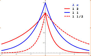
In probability theory and statistics, the asymmetric Laplace distribution (ALD) is a continuous probability distribution which is a generalization of the Laplace distribution. Just as the Laplace distribution consists of two exponential distributions of equal scale back-to-back about x = m, the asymmetric Laplace consists of two exponential distributions of unequal scale back to back about x = m, adjusted to assure continuity and normalization. The difference of two variates exponentially distributed with different means and rate parameters will be distributed according to the ALD. When the two rate parameters are equal, the difference will be distributed according to the Laplace distribution.

In probability theory and statistics, the discrete Weibull distribution is the discrete variant of the Weibull distribution. It was first described by Nakagawa and Osaki in 1975.

In econometrics, the truncated normal hurdle model is a variant of the Tobit model and was first proposed by Cragg in 1971.

References

  1. Hayashi, Fumio (2000). Econometrics . Princeton: Princeton University Press. pp.  518–521. ISBN   0-691-01018-8.
  2. Goldberger, Arthur S. (1964). Econometric Theory . New York: J. Wiley. pp.  253–55. ISBN   9780471311010.
  3. Tobin, James (1958). "Estimation of Relationships for Limited Dependent Variables" (PDF). Econometrica. 26 (1): 24–36. doi:10.2307/1907382. JSTOR   1907382.
  4. Amemiya, Takeshi (1984). "Tobit Models: A Survey". Journal of Econometrics . 24 (1–2): 3–61. doi:10.1016/0304-4076(84)90074-5.
  5. Kennedy, Peter (2003). A Guide to Econometrics (Fifth ed.). Cambridge: MIT Press. pp. 283–284. ISBN   0-262-61183-X.
  6. Bierens, Herman J. (2004). Introduction to the Mathematical and Statistical Foundations of Econometrics . Cambridge University Press. p.  207.
  7. Olsen, Randall J. (1978). "Note on the Uniqueness of the Maximum Likelihood Estimator for the Tobit Model". Econometrica . 46 (5): 1211–1215. doi:10.2307/1911445. JSTOR   1911445.
  8. Orme, Chris (1989). "On the Uniqueness of the Maximum Likelihood Estimator in Truncated Regression Models". Econometric Reviews. 8 (2): 217–222. doi:10.1080/07474938908800171.
  9. Iwata, Shigeru (1993). "A Note on Multiple Roots of the Tobit Log Likelihood". Journal of Econometrics . 56 (3): 441–445. doi:10.1016/0304-4076(93)90129-S.
  10. Amemiya, Takeshi (1973). "Regression analysis when the dependent variable is truncated normal". Econometrica . 41 (6): 997–1016. doi:10.2307/1914031. JSTOR   1914031.
  11. McDonald, John F.; Moffit, Robert A. (1980). "The Uses of Tobit Analysis". The Review of Economics and Statistics . 62 (2): 318–321. doi:10.2307/1924766. JSTOR   1924766.
  12. Schnedler, Wendelin (2005). "Likelihood estimation for censored random vectors" (PDF). Econometric Reviews. 24 (2): 195–217. doi:10.1081/ETC-200067925. hdl:10419/127228. S2CID   55747319.
  13. Amemiya, Takeshi (1985). "Tobit Models". Advanced econometrics . Cambridge, Mass: Harvard University Press. p.  384. ISBN   0-674-00560-0. OCLC   11728277.
  14. Heckman, James J. (1979). "Sample Selection Bias as a Specification Error". Econometrica. 47 (1): 153–161. doi:10.2307/1912352. ISSN   0012-9682. JSTOR   1912352.
  15. Sigelman, Lee; Zeng, Langche (1999). "Analyzing Censored and Sample-Selected Data with Tobit and Heckit Models". Political Analysis. 8 (2): 167–182. doi:10.1093/oxfordjournals.pan.a029811. ISSN   1047-1987. JSTOR   25791605.
  16. Powell, James L (1 July 1984). "Least absolute deviations estimation for the censored regression model". Journal of Econometrics. 25 (3): 303–325. CiteSeerX   10.1.1.461.4302 . doi:10.1016/0304-4076(84)90004-6.
  17. Dahlberg, Matz; Johansson, Eva (2002-03-01). "On the Vote-Purchasing Behavior of Incumbent Governments". American Political Science Review. 96 (1): 27–40. CiteSeerX   10.1.1.198.4112 . doi:10.1017/S0003055402004215. ISSN   1537-5943. S2CID   12718473.
  18. Dubois, Hans F. W.; Fattore, Giovanni (2011-07-01). "Public Fund Assignment through Project Evaluation". Regional & Federal Studies. 21 (3): 355–374. doi:10.1080/13597566.2011.578827. ISSN   1359-7566. S2CID   154659642.
  19. Baltas, George (2001). "Utility-consistent Brand Demand Systems with Endogenous Category Consumption: Principles and Marketing Applications". Decision Sciences. 32 (3): 399–422. doi:10.1111/j.1540-5915.2001.tb00965.x. ISSN   0011-7315.

Further reading