In the mathematical subfield numerical analysis, tricubic interpolation is a method for obtaining values at arbitrary points in 3D space of a function defined on a regular grid. The approach involves approximating the function locally by an expression of the form
This form has 64 coefficients ; requiring the function to have a given value or given directional derivative at a point places one linear constraint on the 64 coefficients.
The term tricubic interpolation is used in more than one context; some experiments measure both the value of a function and its spatial derivatives, and it is desirable to interpolate preserving the values and the measured derivatives at the grid points. Those provide 32 constraints on the coefficients, and another 32 constraints can be provided by requiring smoothness of higher derivatives. [1]
In other contexts, we can obtain the 64 coefficients by considering a 3×3×3 grid of small cubes surrounding the cube inside which we evaluate the function, and fitting the function at the 64 points on the corners of this grid.
The cubic interpolation article indicates that the method is equivalent to a sequential application of one-dimensional cubic interpolators. Let be the value of a monovariable cubic polynomial (e.g. constrained by values, , , , from consecutive grid points) evaluated at . In many useful cases, these cubic polynomials have the form for some vector which is a function of alone. The tricubic interpolator is equivalent to:
where and .
At first glance, it might seem more convenient to use the 21 calls to described above instead of the matrix described in Lekien and Marsden. [1] However, a proper implementation using a sparse format for the matrix (that is fairly sparse) makes the latter more efficient. This aspect is even much more pronounced when interpolation is needed at several locations inside the same cube. In this case, the matrix is used once to compute the interpolation coefficients for the entire cube. The coefficients are then stored and used for interpolation at any location inside the cube. In comparison, sequential use of one-dimensional integrators performs extremely poorly for repeated interpolations because each computational step must be repeated for each new location.
In the mathematical field of numerical analysis, interpolation is a type of estimation, a method of constructing (finding) new data points based on the range of a discrete set of known data points.
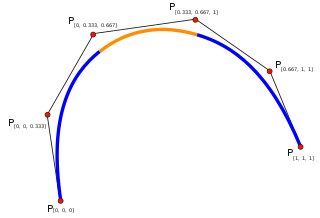
In the mathematical subfield of numerical analysis, a B-spline or basis spline is a spline function that has minimal support with respect to a given degree, smoothness, and domain partition. Any spline function of given degree can be expressed as a linear combination of B-splines of that degree. Cardinal B-splines have knots that are equidistant from each other. B-splines can be used for curve-fitting and numerical differentiation of experimental data.
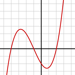
In algebra, a cubic equation in one variable is an equation of the form
The Chebyshev polynomials are two sequences of polynomials related to the cosine and sine functions, notated as and . They can be defined in several equivalent ways, one of which starts with trigonometric functions:
In numerical analysis, polynomial interpolation is the interpolation of a given bivariate data set by the polynomial of lowest possible degree that passes through the points of the dataset.
In the mathematical field of numerical analysis, a Newton polynomial, named after its inventor Isaac Newton, is an interpolation polynomial for a given set of data points. The Newton polynomial is sometimes called Newton's divided differences interpolation polynomial because the coefficients of the polynomial are calculated using Newton's divided differences method.
In mathematics, the beta function, also called the Euler integral of the first kind, is a special function that is closely related to the gamma function and to binomial coefficients. It is defined by the integral
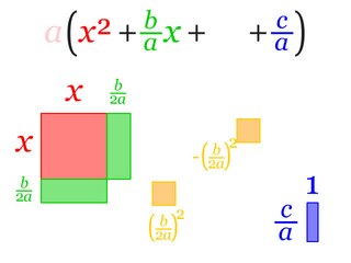
In elementary algebra, completing the square is a technique for converting a quadratic polynomial of the form
In mathematics, a spline is a special function defined piecewise by polynomials. In interpolating problems, spline interpolation is often preferred to polynomial interpolation because it yields similar results, even when using low degree polynomials, while avoiding Runge's phenomenon for higher degrees.
In numerical analysis, a cubic Hermite spline or cubic Hermite interpolator is a spline where each piece is a third-degree polynomial specified in Hermite form, that is, by its values and first derivatives at the end points of the corresponding domain interval.
In mathematics, trigonometric interpolation is interpolation with trigonometric polynomials. Interpolation is the process of finding a function which goes through some given data points. For trigonometric interpolation, this function has to be a trigonometric polynomial, that is, a sum of sines and cosines of given periods. This form is especially suited for interpolation of periodic functions.
In mathematics, the Riesz–Thorin theorem, often referred to as the Riesz–Thorin interpolation theorem or the Riesz–Thorin convexity theorem, is a result about interpolation of operators. It is named after Marcel Riesz and his student G. Olof Thorin.
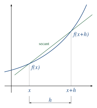
In numerical analysis, numerical differentiation algorithms estimate the derivative of a mathematical function or function subroutine using values of the function and perhaps other knowledge about the function.
In mathematics, Birkhoff interpolation is an extension of polynomial interpolation. It refers to the problem of finding a polynomial of degree such that only certain derivatives have specified values at specified points:
A Savitzky–Golay filter is a digital filter that can be applied to a set of digital data points for the purpose of smoothing the data, that is, to increase the precision of the data without distorting the signal tendency. This is achieved, in a process known as convolution, by fitting successive sub-sets of adjacent data points with a low-degree polynomial by the method of linear least squares. When the data points are equally spaced, an analytical solution to the least-squares equations can be found, in the form of a single set of "convolution coefficients" that can be applied to all data sub-sets, to give estimates of the smoothed signal, at the central point of each sub-set. The method, based on established mathematical procedures, was popularized by Abraham Savitzky and Marcel J. E. Golay, who published tables of convolution coefficients for various polynomials and sub-set sizes in 1964. Some errors in the tables have been corrected. The method has been extended for the treatment of 2- and 3-dimensional data.
In numerical analysis, Hermite interpolation, named after Charles Hermite, is a method of polynomial interpolation, which generalizes Lagrange interpolation. Lagrange interpolation allows computing a polynomial of degree less than n that takes the same value at n given points as a given function. Instead, Hermite interpolation computes a polynomial of degree less than mn such that the polynomial and its m − 1 first derivatives have the same values at n given points as a given function and its m − 1 first derivatives.
Lanczos filtering and Lanczos resampling are two applications of a mathematical formula. It can be used as a low-pass filter or used to smoothly interpolate the value of a digital signal between its samples. In the latter case, it maps each sample of the given signal to a translated and scaled copy of the Lanczos kernel, which is a sinc function windowed by the central lobe of a second, longer, sinc function. The sum of these translated and scaled kernels is then evaluated at the desired points.
In applied mathematics, polyharmonic splines are used for function approximation and data interpolation. They are very useful for interpolating and fitting scattered data in many dimensions. Special cases include thin plate splines and natural cubic splines in one dimension.
In numerical analysis, multivariate interpolation is interpolation on functions of more than one variable ; when the variates are spatial coordinates, it is also known as spatial interpolation.
Barnes interpolation, named after Stanley L. Barnes, is the interpolation of unevenly spread data points from a set of measurements of an unknown function in two dimensions into an analytic function of two variables. An example of a situation where the Barnes scheme is important is in weather forecasting where measurements are made wherever monitoring stations may be located, the positions of which are constrained by topography. Such interpolation is essential in data visualisation, e.g. in the construction of contour plots or other representations of analytic surfaces.