ZOOMQ3D

Last updated

ZOOMQ3D is a numerical finite-difference model, which simulates groundwater flow in aquifers. The program is used by hydrogeologists to investigate groundwater resources and to make predictions about possible future changes in their quantity and quality. The code is written in C++, an object-oriented programming language and can compile and run on Windows and Unix operating systems.

Contents

Groundwater flow equation

ZOOMQ3D applies a quasi-three-dimensional finite-difference approximation to the general three-dimensional governing partial differential groundwater flow equation:

where:

This equation is derived by considering a flow balance for an infinitesimally small volume element located anywhere within a body of saturated aquifer. A number of assumptions underlie this equation. First, the fluid is assumed to be of constant density; this allows the flow balance to be a consequence of mass conservation within the element. Next, the Cartesian coordinate system is aligned with the principal axes of the hydraulic conductivity tensor; this avoids the need for cross derivatives.

A model, based on the above equation, incorporating appropriate boundary and initial conditions, would be truly three-dimensional. ZOOMQ3D takes a simplifying approach to the solution of the three-dimensional equation by recognising that in many aquifers it is possible to identify a layered structure. If the layers are aligned parallel to the horizontal coordinate axes, then the three-dimensional equation can be integrated vertically across the layer to produce an equation which describes the flow within a layer and its interactions with adjacent layers. Such an equation is:

where:

Model features

FeatureDescription
Multiple layersZOOMQ3D can incorporate multiple layers of finite difference nodes. The elevation of these layers can vary across the model and the base elevation of one layer can be higher than the top of the layer below it. The separation of model layers simplifies the representation of groundwater systems that contain aquifers separated aquitards. This because the flow through low permeability layers, which is assumed to be vertical, is represented by the vertical leakage term connecting two finite difference nodes within the upper and lower aquifer.
Local grid refinementZOOMQ3D incorporates a mesh refinement procedure which aids the solution of problems related to scale. The density of finite difference nodes can be increased by adding successively finer rectangular grids in discrete areas of the model domain. The mesh can be refined in separate areas and grids can be refined multiple times in the same location in order to zoom into a specific model feature, for example an abstraction borehole or a river reach.
Confined - unconfined conditionsBoth confined and unconfined aquifers can be modelled. At confined finite difference nodes transmissivity and storage are independent of groundwater head. At unconfined nodes transmissivity is a function of saturated thickness and the storage term incorporates specific yield. In the top model layer finite different nodes can be defined as being confined, unconfined or convertible. Convertible nodes switch between unconfined and confined behaviour when the groundwater head rises above its top elevation. In each of the lower model layers, all the nodes must be specified as being either confined or convertible.

Finite difference nodes dewater as the groundwater head drops below their base. In this case the node is removed from the matrix of finite difference equations.

Heterogeneity and anisotropyModels can be heterogeneous and anisotropic. Different hydraulic parameter values can be specified at each finite difference node and hydraulic conductivity may be different in the x and y-directions. It is assumed that the Cartesian co-ordinate system is aligned with the principal axes of the hydraulic conductivity tensor.
Moving boundariesModel nodes can de-water and re-wet. Nodes are made inactive when the groundwater level falls below their base and vice versa. The re-wetting of model nodes depends on the groundwater head in adjacent finite difference nodes.
Variable hydraulic conductivity with depth (VKD)Vertical variations in hydraulic conductivity with depth can be specified within model layers or across model layers by defining VKD profiles. The transmissivity at a node is calculated by integrating the hydraulic conductivity over the vertical saturated thickness of the node.
RechargeRecharge can vary spatially and temporally. Recharge is always applied to the upper-most active node.
Abstraction wellsPumped boreholes can be placed at any node within the model domain. Abstraction rates can vary temporally and wells can both abstract water from the aquifer and inject water into it.
RiversDendritic rivers basins are simulated using a series of interconnected river reaches. The hydraulic parameters characterising a reach can vary along the river as can the degree of connection with the aquifer. The transfer of water between the aquifer and rivers is simulated as is the accretion of baseflow along each river branch. Discharges to the river can be specified in any reach, for example to represent a sewage treatment works, and the discharge rate can vary over time. Both fully penetrating and perched rivers can be simulated.
Head-dependent leakage nodesIn addition to rivers, a second head-dependent leakage mechanism is included in ZOOMQ3D. The flow through leakage nodes is proportional to the difference between its elevation and the groundwater head at the finite difference node to which it is connected. Flow can occur in either direction i.e. into or out of the aquifer. Leakage nodes can be used to model spring flows, lakes or estuaries, for example.
SpringsThis model feature has been developed to simulated spring flows specifically. The flow out of a spring depends on the transmissivity of the surrounding finite difference nodes. Spring flows are represented by an ‘abstraction’ which removes water from the aquifer at the location of the spring until the water table falls below the level of the ground surface.
Time discretisationSimulation time is divided into time-steps, stress periods and blocks. The length of a time-step is equivalent to the length of time between which successive solutions are calculated for the model's state variables. A stress period represents a period of time during which all model stresses remain constant e.g. recharge, groundwater abstraction or discharge to rivers. Stress periods are divided into one or more time-steps. A block is composed of one or more stress periods. The rationale for the use of blocks is predominantly related to the simplification of the organisation of time-variant data, for example, groundwater abstraction or recharge rates, within input files. The number of stress periods in each block is the same for all blocks within a simulation.

History of development

The groundwater flow model ZOOMQ3D is one of the codes in the ZOOM family of numerical groundwater models which also consists of the advective transport particle tracking code ZOOPT and the distributed recharge model ZOODRM. Each of these models has been developed using object-oriented techniques, a programming approach commonly applied in commercial software development but only relatively recently adopted in numerical modelling for scientific analysis.

ZOOMQ3D and ZOOPT have been developed through a tri-partite collaboration between the School of Civil Engineering of the University of Birmingham, UK, the British Geological Survey and the Environment Agency of England and Wales. The distributed recharge model ZOODRM has been developed by the British Geological Survey. All models are maintained by the British Geological Survey.

A link exists between ZOOMQ3D and the geological modelling software GSI3D. The link facilitates the transfer of the structure of a geological model into a ZOOMQ3D groundwater model. After a GSI3D geological model is constructed it can be used to create a hydrogeological model of an aquifer. This is achieved by assigning hydrogeological parameters, such as hydraulic conductivity, to the geological units. Once this has been completed the resulting hydrogeological model can then be converted to a layered ZOOMQ3D groundwater model.

Related Research Articles

Laplaces equation Second order partial differential equation

In mathematics and physics, Laplace's equation is a second-order partial differential equation named after Pierre-Simon Laplace, who first studied its properties. This is often written as

Navier–Stokes equations Equations describing the motion of viscous fluid substances

In physics, the Navier–Stokes equations are certain partial differential equations which describe the motion of viscous fluid substances, named after French engineer and physicist Claude-Louis Navier and Anglo-Irish physicist and mathematician George Gabriel Stokes. They were developed over several decades of progressively building the theories, from 1822 (Navier) to 1842–1850 (Stokes).
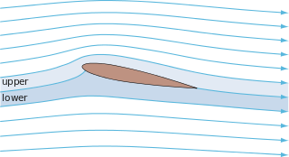
Potential flow Velocity field as the gradient of a scalar function

In fluid dynamics, potential flow describes the velocity field as the gradient of a scalar function: the velocity potential. As a result, a potential flow is characterized by an irrotational velocity field, which is a valid approximation for several applications. The irrotationality of a potential flow is due to the curl of the gradient of a scalar always being equal to zero.

Heat equation Type of partial differential equation

In mathematics and physics, the heat equation is a certain partial differential equation. Solutions of the heat equation are sometimes known as caloric functions. The theory of the heat equation was first developed by Joseph Fourier in 1822 for the purpose of modeling how a quantity such as heat diffuses through a given region.

Poissons equation Expression frequently encountered in mathematical physics, generalization of Laplaces equation.

Poisson's equation is an elliptic partial differential equation of broad utility in theoretical physics. For example, the solution to Poisson's equation is the potential field caused by a given electric charge or mass density distribution; with the potential field known, one can then calculate electrostatic or gravitational (force) field. It is a generalization of Laplace's equation, which is also frequently seen in physics. The equation is named after French mathematician and physicist Siméon Denis Poisson.

Darcy's law is an equation that describes the flow of a fluid through a porous medium. The law was formulated by Henry Darcy based on results of experiments on the flow of water through beds of sand, forming the basis of hydrogeology, a branch of earth sciences. It is analogous to Ohm's law in electrostatics, linearly relating the volume flow rate of the fluid to the hydraulic head difference via the hydraulic conductivity.

Large eddy simulation

Large eddy simulation (LES) is a mathematical model for turbulence used in computational fluid dynamics. It was initially proposed in 1963 by Joseph Smagorinsky to simulate atmospheric air currents, and first explored by Deardorff (1970). LES is currently applied in a wide variety of engineering applications, including combustion, acoustics, and simulations of the atmospheric boundary layer.

Nonlinear Schrödinger equation

In theoretical physics, the (one-dimensional) nonlinear Schrödinger equation (NLSE) is a nonlinear variation of the Schrödinger equation. It is a classical field equation whose principal applications are to the propagation of light in nonlinear optical fibers and planar waveguides and to Bose–Einstein condensates confined to highly anisotropic cigar-shaped traps, in the mean-field regime. Additionally, the equation appears in the studies of small-amplitude gravity waves on the surface of deep inviscid (zero-viscosity) water; the Langmuir waves in hot plasmas; the propagation of plane-diffracted wave beams in the focusing regions of the ionosphere; the propagation of Davydov's alpha-helix solitons, which are responsible for energy transport along molecular chains; and many others. More generally, the NLSE appears as one of universal equations that describe the evolution of slowly varying packets of quasi-monochromatic waves in weakly nonlinear media that have dispersion. Unlike the linear Schrödinger equation, the NLSE never describes the time evolution of a quantum state. The 1D NLSE is an example of an integrable model.

Used in hydrogeology, the groundwater flow equation is the mathematical relationship which is used to describe the flow of groundwater through an aquifer. The transient flow of groundwater is described by a form of the diffusion equation, similar to that used in heat transfer to describe the flow of heat in a solid. The steady-state flow of groundwater is described by a form of the Laplace equation, which is a form of potential flow and has analogs in numerous fields.

MODFLOW

MODFLOW is the U.S. Geological Survey modular finite-difference flow model, which is a computer code that solves the groundwater flow equation. The program is used by hydrogeologists to simulate the flow of groundwater through aquifers. The source code is free public domain software, written primarily in Fortran, and can compile and run on Microsoft Windows or Unix-like operating systems.

Eddy diffusion

Eddy diffusion, eddy dispersion, or turbulent diffusion is a process by which substances are mixed in the atmosphere, the ocean or in any fluid system due to eddy motion. In other words, it is mixing that is caused by eddies that can vary in size from subtropical ocean gyres down to the small Kolmogorov microscales. The concept of turbulence or turbulent flow causes eddy diffusion to occur. The theory of eddy diffusion was first developed by Sir Geoffrey Ingram Taylor.

Groundwater discharge is the volumetric flow rate of groundwater through an aquifer.

The intent of this article is to highlight the important points of the derivation of the Navier–Stokes equations as well as its application and formulation for different families of fluids.

HydroGeoSphere

HydroGeoSphere (HGS) is a 3D control-volume finite element groundwater model, and is based on a rigorous conceptualization of the hydrologic system consisting of surface and subsurface flow regimes. The model is designed to take into account all key components of the hydrologic cycle. For each time step, the model solves surface and subsurface flow, solute and energy transport equations simultaneously, and provides a complete water and solute balance.

The Cauchy momentum equation is a vector partial differential equation put forth by Cauchy that describes the non-relativistic momentum transport in any continuum.

Gravitational lensing formalism

In general relativity, a point mass deflects a light ray with impact parameter by an angle approximately equal to

Mild-slope equation Physics phenomenon and formula

In fluid dynamics, the mild-slope equation describes the combined effects of diffraction and refraction for water waves propagating over bathymetry and due to lateral boundaries—like breakwaters and coastlines. It is an approximate model, deriving its name from being originally developed for wave propagation over mild slopes of the sea floor. The mild-slope equation is often used in coastal engineering to compute the wave-field changes near harbours and coasts.

In mathematics, the method of steepest descent or saddle-point method is an extension of Laplace's method for approximating an integral, where one deforms a contour integral in the complex plane to pass near a stationary point, in roughly the direction of steepest descent or stationary phase. The saddle-point approximation is used with integrals in the complex plane, whereas Laplace’s method is used with real integrals.

In the study of differential equations, the Loewy decomposition breaks every linear ordinary differential equation (ODE) into what are called largest completely reducible components. It was introduced by Alfred Loewy.

The Marine Unsaturated Model is a two-dimensional finite element model capable of simulating the migration of water and solutes in saturated-unsaturated porous media while accounting for the impact of solute concentration on water density and viscosity, as saltwater is heaving and more viscous than freshwater. The detailed formulation of the MARUN model is found in and. The model was used to investigate seepage flow in trenches and dams, the migration of brine following evaporation and, submarine groundwater discharge, and beach hydrodynamics to explain the persistence of some of the Exxon Valdez oil in Alaska beaches.

References