Blade element momentum theory is a theory that combines both blade element theory and momentum theory. It is used to calculate the local forces on a propeller or wind-turbine blade. Blade element theory is combined with momentum theory to alleviate some of the difficulties in calculating the induced velocities at the rotor.
This article emphasizes application of blade element theory to ground-based wind turbines, but the principles apply as well to propellers. Whereas the streamtube area is reduced by a propeller, it is expanded by a wind turbine. For either application, a highly simplified but useful approximation is the Rankine–Froude "momentum" or "actuator disk" model (1865,[1] 1889[2]). This article explains the application of the "Betz limit" to the efficiency of a ground-based wind turbine.
Froude's blade element theory (1878)[3] is a mathematical process to determine the behavior of propellers, later refined by Glauert (1926). Betz (1921) provided an approximate correction to momentum "Rankine–Froude actuator-disk" theory [4] to account for the sudden rotation imparted to the flow by the actuator disk (NACA TN 83, "The Theory of the Screw Propeller" and NACA TM 491, "Propeller Problems"). In blade element momentum theory, angular momentum is included in the model, meaning that the wake (the air after interaction with the rotor) has angular momentum. That is, the air begins to rotate about the z-axis immediately upon interaction with the rotor (see diagram below). Angular momentum must be taken into account since the rotor, which is the device that extracts the energy from the wind, is rotating as a result of the interaction with the wind.
Rankine–Froude model
The "Betz limit," not yet taking advantage of Betz' contribution to account for rotational flow with emphasis on propellers, applies the Rankine–Froude "actuator disk" theory to obtain the maximum efficiency of a stationary wind turbine. The following analysis is restricted to axial motion of the air:
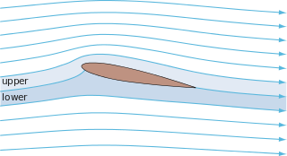
In our streamtube we have fluid flowing from left to right, and an actuator disk that represents the rotor. We will assume that the rotor is infinitesimally thin.[5] From above, we can see that at the start of the streamtube, fluid flow is normal to the actuator disk. The fluid interacts with the rotor, thus transferring energy from the fluid to the rotor. The fluid then continues to flow downstream. Thus we can break our system/streamtube into two sections: pre-acuator disk, and post-actuator disk. Before interaction with the rotor, the total energy in the fluid is constant. Furthermore, after interacting with the rotor, the total energy in the fluid is constant.
Bernoulli's equation describes the different forms of energy that are present in fluid flow where the net energy is constant, i.e. when a fluid is not transferring any energy to some other entity such as a rotor. The energy consists of static pressure, gravitational potential energy, and kinetic energy. Mathematically, we have the following expression:
where is the density of the fluid, is the velocity of the fluid along a streamline, is the static pressure energy, is the acceleration due to gravity, and is the height above the ground. For the purposes of this analysis, we will assume that gravitational potential energy is unchanging during fluid flow from left to right such that we have the following:
Thus, if we have two points on a streamline, point 1 and point 2, and at point 1 the velocity of the fluid along the streamline is and the pressure at 1 is , and at point 2 the velocity of the fluid along the streamline is and the pressure at 2 is , and no energy has been extracted from the fluid between points 1 and 2, then we have the following expression:
Now let us return to our initial diagram. Consider pre-actuator flow. Far upstream, the fluid velocity is ; the fluid velocity then decreases and pressure increases as it approaches the rotor.[4] In accordance with mass conservation, the mass flow rate through the rotor must be constant. The mass flow rate, , through a surface of area is given by the following expression:
where is the density and is the velocity of the fluid along a streamline. Thus, if mass flow rate is constant, increases in area must result in decreases in fluid velocity along a streamline. This means the kinetic energy of the fluid is decreasing. If the flow is expanding but not transferring energy, then Bernoulli applies. Thus the reduction in kinetic energy is countered by an increase in static pressure energy.
So we have the following situation pre-rotor: far upstream, fluid pressure is the same as atmospheric, ; just before interaction with the rotor, fluid pressure has increased and so kinetic energy has decreased. This can be described mathematically using Bernoulli's equation:
where we have written the fluid velocity at the rotor as , where is the axial induction factor. The pressure of the fluid on the upstream side of the actuator disk is . We are treating the rotor as an actuator disk that is infinitely thin. Thus we will assume no change in fluid velocity across the actuator disk. Since energy has been extracted from the fluid, the pressure must have decreased.
Now consider post-rotor: immediately after interacting with the rotor, the fluid velocity is still , but the pressure has dropped to a value ; far downstream, pressure of the fluid has reached equilibrium with the atmosphere; this has been accomplished in the natural and dynamically slow process of decreasing the velocity of flow in the stream tube in order to maintain dynamic equilibrium ( i.e. far downstream. Assuming no further energy transfer, we can apply Bernoulli for downstream:
where
The velocity far downstream in the Wake
Thus we can obtain an expression for the pressure difference between fore and aft of the rotor:
If we have a pressure difference across the area of the actuator disc, there is a force acting on the actuator disk, which can be determined from :
where is the area of the actuator disk. If the rotor is the only thing absorbing energy from the fluid, the rate of change in axial momentum of the fluid is the force that is acting on the rotor. The rate of change of axial momentum can be expressed as the difference between the initial and final axial velocities of the fluid, multiplied by the mass flow rate:
Thus we can arrive at an expression for the fluid velocity far downstream:
This force is acting at the rotor. The power taken from the fluid is the force acting on the fluid multiplied by the velocity of the fluid at the point of power extraction:
Maximum power
Suppose we are interested in finding the maximum power that can be extracted from the fluid. The power in the fluid is given by the following expression:
where is the fluid density as before, is the fluid velocity, and is the area of an imaginary surface through which the fluid is flowing. The power extracted from the fluid by a rotor in the scenario described above is some fraction of this power expression. We will call the fraction the power co-efficient, . Thus the power extracted, is given by the following expression:
Our question is this: what is the maximum value of using the Betz model?
Let us return to our derived expression for the power transferred from the fluid to the rotor (). We can see that the power extracted is dependent on the axial induction factor. If we differentiate with respect to , we get the following result:
If we have maximised our power extraction, we can set the above to zero. This allows us to determine the value of which yields maximum power extraction. This value is a . Thus we are able to find that . In other words, the rotor cannot extract more than 59 per cent of the power in the fluid.
Blade element momentum theory
Compared to the Rankine–Froude model, Blade element momentum theory accounts for the angular momentum of the rotor. Consider the left hand side of the figure below. We have a streamtube, in which there is the fluid and the rotor. We will assume that there is no interaction between the contents of the streamtube and everything outside of it. That is, we are dealing with an isolated system. In physics, isolated systems must obey conservation laws. An example of such is the conservation of angular momentum. Thus, the angular momentum within the streamtube must be conserved. Consequently, if the rotor acquires angular momentum through its interaction with the fluid, something else must acquire equal and opposite angular momentum. As already mentioned, the system consists of just the fluid and the rotor, the fluid must acquire angular momentum in the wake. As we related the change in axial momentum with some induction factor , we will relate the change in angular momentum of the fluid with the tangential induction factor, .
We will break the rotor area up into annular rings of infinitesimally small thickness. We are doing this so that we can assume that axial induction factors and tangential induction factors are constant throughout the annular ring. An assumption of this approach is that annular rings are independent of one another i.e. there is no interaction between the fluids of neighboring annular rings.
Bernoulli for rotating wake
Let us now go back to Bernoulli:
The velocity is the velocity of the fluid along a streamline. The streamline may not necessarily run parallel to a particular co-ordinate axis, such as the z-axis. Thus the velocity may consist of components in the axes that make up the co-ordinate system. For this analysis, we will use cylindrical polar co-ordinates . Thus .
NOTE: We will in fact, be working in cylindrical co-ordinates for all aspects e.g.
Now consider the setup shown above. As before, we can break the setup into two components: upstream and downstream.
Pre-rotor
where is the velocity of the fluid along a streamline far upstream, and is the velocity of the fluid just prior to the rotor. Written in cylindrical polar co-ordinates, we have the following expression:
where and are the z-components of the velocity far upstream and just prior to the rotor respectively. This is exactly the same as the upstream equation from the Betz model.
As can be seen from the figure above, the flow expands as it approaches the rotor, a consequence of the increase in static pressure and the conservation of mass. This would imply that upstream. However, for the purpose of this analysis, that effect will be neglected.
Post-rotor
where is the velocity of the fluid just after interacting with the rotor. This can be written as . The radial component of the velocity will be zero; this must be true if we are to use the annular ring approach; to assume otherwise would suggest interference between annular rings at some point downstream. Since we assume that there is no change in axial velocity across the disc, . Angular momentum must be conserved in an isolated system. Thus the rotation of the wake must not die away. Thus in the downstream section is constant. Thus Bernoulli simplifies in the downstream section:
In other words, the Bernoulli equations up and downstream of the rotor are the same as the Bernoulli expressions in the Betz model. Therefore, we can use results such as power extraction and wake speed that were derived in the Betz model i.e.
This allows us to calculate maximum power extraction for a system that includes a rotating wake. This can be shown to give the same value as that of the Betz model i.e. 0.59. This method involves recognising that the torque generated in the rotor is given by the following expression:
with the necessary terms defined immediately below.
Blade forces
Consider fluid flow around an airfoil. The flow of the fluid around the airfoil gives rise to lift and drag forces. By definition, lift is the force that acts on the airfoil normal to the apparent fluid flow speed seen by the airfoil. Drag is the forces that acts tangential to the apparent fluid flow speed seen by the airfoil. What do we mean by an apparent speed? Consider the diagram below:
The speed seen by the rotor blade is dependent on three things: the axial velocity of the fluid, ; the tangential velocity of the fluid due to the acceleration round an airfoil, ; and the rotor motion itself, . That is, the apparent fluid velocity is given as below:
Thus the apparent wind speed is just the magnitude of this vector i.e.:
We can also work out the angle from the above figure:
Supposing we know the angle , we can then work out simply by using the relation ; we can then work out the lift co-efficient, , and the drag co-efficient , from which we can work out the lift and drag forces acting on the blade.
Consider the annular ring, which is partially occupied by blade elements. The length of each blade section occupying the annular ring is (see figure below).
The lift acting on those parts of the blades/airfoils each with chord is given by the following expression:
where is the lift co-efficient, which is a function of the angle of attack, and is the number of blades. Additionally, the drag acting on that part of the blades/airfoils with chord is given by the following expression:
Remember that these forces calculated are normal and tangential to the apparent speed. We are interested in forces in the and axes. Thus we need to consider the diagram below:
Thus we can see the following:
is the force that is responsible for the rotation of the rotor blades; is the force that is responsible for the bending of the blades.
Recall that for an isolated system the net angular momentum of the system is conserved. If the rotor acquired angular momentum, so must the fluid in the wake. Let us suppose that the fluid in the wake acquires a tangential velocity . Thus the torque in the air is given by
By the conservation of angular momentum, this balances the torque in the blades of the rotor; thus,
Furthermore, the rate of change of linear momentum in the air is balanced by the out-of-plane bending force acting on the blades, . From momentum theory, the rate of change of linear momentum in the air is as follows:
which may be expressed as
Balancing this with the out-of-plane bending force gives
Let us now make the following definitions:
So we have the following equations:
(1)
(2)
Let us make reference to the following equation which can be seen from analysis of the above figure:
(3)
Thus, with these three equations, it is possible to get the following result through some algebraic manipulation:[5]
We can derive an expression for in a similar manner. This allows us to understand what is going on with the rotor and the fluid. Equations of this sort are then solved by iterative techniques.
Assumptions and possible drawbacks of BEM models
Assumes that each annular ring is independent of every other annular ring.[6]
Does not account for wake expansion.
Does not account for tip losses, though correction factors can be included.[7]
Does not account for yaw, though it can be made to do so.
Based on steady flow (non-turbulent).
Related Research Articles
The Navier–Stokes equations are partial differential equations which describe the motion of viscous fluid substances, named after French engineer and physicist Claude-Louis Navier and Irish physicist and mathematician George Gabriel Stokes. They were developed over several decades of progressively building the theories, from 1822 (Navier) to 1842-1850 (Stokes).
In fluid dynamics, potential flow describes the velocity field as the gradient of a scalar function: the velocity potential. As a result, a potential flow is characterized by an irrotational velocity field, which is a valid approximation for several applications. The irrotationality of a potential flow is due to the curl of the gradient of a scalar always being equal to zero.
Bernoulli's principle is a key concept in fluid dynamics that relates pressure, speed and height. Bernoulli's principle states that an increase in the speed of a fluid occurs simultaneously with a decrease in static pressure or the fluid's potential energy. The principle is named after the Swiss mathematician and physicist Daniel Bernoulli, who published it in his book Hydrodynamica in 1738. Although Bernoulli deduced that pressure decreases when the flow speed increases, it was Leonhard Euler in 1752 who derived Bernoulli's equation in its usual form.
The stress–energy tensor, sometimes called the stress–energy–momentum tensor or the energy–momentum tensor, is a tensor physical quantity that describes the density and flux of energy and momentum in spacetime, generalizing the stress tensor of Newtonian physics. It is an attribute of matter, radiation, and non-gravitational force fields. This density and flux of energy and momentum are the sources of the gravitational field in the Einstein field equations of general relativity, just as mass density is the source of such a field in Newtonian gravity.
Particle velocity is the velocity of a particle in a medium as it transmits a wave. The SI unit of particle velocity is the metre per second (m/s). In many cases this is a longitudinal wave of pressure as with sound, but it can also be a transverse wave as with the vibration of a taut string.
Large eddy simulation (LES) is a mathematical model for turbulence used in computational fluid dynamics. It was initially proposed in 1963 by Joseph Smagorinsky to simulate atmospheric air currents, and first explored by Deardorff (1970). LES is currently applied in a wide variety of engineering applications, including combustion, acoustics, and simulations of the atmospheric boundary layer.
Stokes flow, also named creeping flow or creeping motion, is a type of fluid flow where advective inertial forces are small compared with viscous forces. The Reynolds number is low, i.e. . This is a typical situation in flows where the fluid velocities are very slow, the viscosities are very large, or the length-scales of the flow are very small. Creeping flow was first studied to understand lubrication. In nature, this type of flow occurs in the swimming of microorganisms and sperm. In technology, it occurs in paint, MEMS devices, and in the flow of viscous polymers generally.
In physics and fluid mechanics, a Blasius boundary layer describes the steady two-dimensional laminar boundary layer that forms on a semi-infinite plate which is held parallel to a constant unidirectional flow. Falkner and Skan later generalized Blasius' solution to wedge flow, i.e. flows in which the plate is not parallel to the flow.
In numerical methods, total variation diminishing (TVD) is a property of certain discretization schemes used to solve hyperbolic partial differential equations. The most notable application of this method is in computational fluid dynamics. The concept of TVD was introduced by Ami Harten.
In the study of partial differential equations, the MUSCL scheme is a finite volume method that can provide highly accurate numerical solutions for a given system, even in cases where the solutions exhibit shocks, discontinuities, or large gradients. MUSCL stands for Monotonic Upstream-centered Scheme for Conservation Laws, and the term was introduced in a seminal paper by Bram van Leer. In this paper he constructed the first high-order, total variation diminishing (TVD) scheme where he obtained second order spatial accuracy.
The Navier–Stokes existence and smoothness problem concerns the mathematical properties of solutions to the Navier–Stokes equations, a system of partial differential equations that describe the motion of a fluid in space. Solutions to the Navier–Stokes equations are used in many practical applications. However, theoretical understanding of the solutions to these equations is incomplete. In particular, solutions of the Navier–Stokes equations often include turbulence, which remains one of the greatest unsolved problems in physics, despite its immense importance in science and engineering.
The Kutta–Joukowski theorem is a fundamental theorem in aerodynamics used for the calculation of lift of an airfoil translating in a uniform fluid at a constant speed large enough so that the flow seen in the body-fixed frame is steady and unseparated. The theorem relates the lift generated by an airfoil to the speed of the airfoil through the fluid, the density of the fluid and the circulation around the airfoil. The circulation is defined as the line integral around a closed loop enclosing the airfoil of the component of the velocity of the fluid tangent to the loop. It is named after Martin Kutta and Nikolai Zhukovsky who first developed its key ideas in the early 20th century. Kutta–Joukowski theorem is an inviscid theory, but it is a good approximation for real viscous flow in typical aerodynamic applications.
In mathematics, the cylindrical harmonics are a set of linearly independent functions that are solutions to Laplace's differential equation, , expressed in cylindrical coordinates, ρ (radial coordinate), φ (polar angle), and z (height). Each function Vn(k) is the product of three terms, each depending on one coordinate alone. The ρ-dependent term is given by Bessel functions (which occasionally are also called cylindrical harmonics).
The Cauchy momentum equation is a vector partial differential equation put forth by Cauchy that describes the non-relativistic momentum transport in any continuum.
In nonideal fluid dynamics, the Hagen–Poiseuille equation, also known as the Hagen–Poiseuille law, Poiseuille law or Poiseuille equation, is a physical law that gives the pressure drop in an incompressible and Newtonian fluid in laminar flow flowing through a long cylindrical pipe of constant cross section. It can be successfully applied to air flow in lung alveoli, or the flow through a drinking straw or through a hypodermic needle. It was experimentally derived independently by Jean Léonard Marie Poiseuille in 1838 and Gotthilf Heinrich Ludwig Hagen, and published by Poiseuille in 1840–41 and 1846. The theoretical justification of the Poiseuille law was given by George Stokes in 1845.
In fluid dynamics, Luke's variational principle is a Lagrangian variational description of the motion of surface waves on a fluid with a free surface, under the action of gravity. This principle is named after J.C. Luke, who published it in 1967. This variational principle is for incompressible and inviscid potential flows, and is used to derive approximate wave models like the mild-slope equation, or using the averaged Lagrangian approach for wave propagation in inhomogeneous media.
f(R) is a type of modified gravity theory which generalizes Einstein's general relativity. f(R) gravity is actually a family of theories, each one defined by a different function, f, of the Ricci scalar, R. The simplest case is just the function being equal to the scalar; this is general relativity. As a consequence of introducing an arbitrary function, there may be freedom to explain the accelerated expansion and structure formation of the Universe without adding unknown forms of dark energy or dark matter. Some functional forms may be inspired by corrections arising from a quantum theory of gravity. f(R) gravity was first proposed in 1970 by Hans Adolph Buchdahl. It has become an active field of research following work by Starobinsky on cosmic inflation. A wide range of phenomena can be produced from this theory by adopting different functions; however, many functional forms can now be ruled out on observational grounds, or because of pathological theoretical problems.
An electric dipole transition is the dominant effect of an interaction of an electron in an atom with the electromagnetic field.
An axial fan is a type of fan that causes gas to flow through it in an axial direction, parallel to the shaft about which the blades rotate. The flow is axial at entry and exit. The fan is designed to produce a pressure difference, and hence force, to cause a flow through the fan. Factors which determine the performance of the fan include the number and shape of the blades. Fans have many applications including in wind tunnels and cooling towers. Design parameters include power, flow rate, pressure rise and efficiency.
Unsteady flows are characterized as flows in which the properties of the fluid are time dependent. It gets reflected in the governing equations as the time derivative of the properties are absent. For Studying Finite-volume method for unsteady flow there is some governing equations >
This page is based on this Wikipedia article Text is available under the CC BY-SA 4.0 license; additional terms may apply. Images, videos and audio are available under their respective licenses.