In economics, the Gini coefficient, also known as the Gini index or Gini ratio, is a measure of statistical dispersion intended to represent the income inequality, the wealth inequality, or the consumption inequality within a nation or a social group. It was developed by Italian statistician and sociologist Corrado Gini.

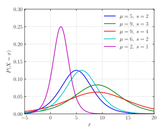
In statistics, a normal distribution or Gaussian distribution is a type of continuous probability distribution for a real-valued random variable. The general form of its probability density function is

The Pareto distribution, named after the Italian civil engineer, economist, and sociologist Vilfredo Pareto, is a power-law probability distribution that is used in description of social, quality control, scientific, geophysical, actuarial, and many other types of observable phenomena; the principle originally applied to describing the distribution of wealth in a society, fitting the trend that a large portion of wealth is held by a small fraction of the population. The Pareto principle or "80-20 rule" stating that 80% of outcomes are due to 20% of causes was named in honour of Pareto, but the concepts are distinct, and only Pareto distributions with shape value of log45 ≈ 1.16 precisely reflect it. Empirical observation has shown that this 80-20 distribution fits a wide range of cases, including natural phenomena and human activities.

In probability theory, a log-normal (or lognormal) distribution is a continuous probability distribution of a random variable whose logarithm is normally distributed. Thus, if the random variable X is log-normally distributed, then Y = ln(X) has a normal distribution. Equivalently, if Y has a normal distribution, then the exponential function of Y, X = exp(Y), has a log-normal distribution. A random variable which is log-normally distributed takes only positive real values. It is a convenient and useful model for measurements in exact and engineering sciences, as well as medicine, economics and other topics (e.g., energies, concentrations, lengths, prices of financial instruments, and other metrics).

In mathematics, Jensen's inequality, named after the Danish mathematician Johan Jensen, relates the value of a convex function of an integral to the integral of the convex function. It was proved by Jensen in 1906, building on an earlier proof of the same inequality for doubly-differentiable functions by Otto Hölder in 1889. Given its generality, the inequality appears in many forms depending on the context, some of which are presented below. In its simplest form the inequality states that the convex transformation of a mean is less than or equal to the mean applied after convex transformation; it is a simple corollary that the opposite is true of concave transformations.
In mathematics, the moments of a function are certain quantitative measures related to the shape of the function's graph. If the function represents mass density, then the zeroth moment is the total mass, the first moment is the center of mass, and the second moment is the moment of inertia. If the function is a probability distribution, then the first moment is the expected value, the second central moment is the variance, the third standardized moment is the skewness, and the fourth standardized moment is the kurtosis. The mathematical concept is closely related to the concept of moment in physics.
Income inequality metrics or income distribution metrics are used by social scientists to measure the distribution of income and economic inequality among the participants in a particular economy, such as that of a specific country or of the world in general. While different theories may try to explain how income inequality comes about, income inequality metrics simply provide a system of measurement used to determine the dispersion of incomes. The concept of inequality is distinct from poverty and fairness.
In probability theory and statistics, the logistic distribution is a continuous probability distribution. Its cumulative distribution function is the logistic function, which appears in logistic regression and feedforward neural networks. It resembles the normal distribution in shape but has heavier tails. The logistic distribution is a special case of the Tukey lambda distribution.
In probability theory and statistics, the coefficient of variation (CV), also known as Normalized Root-Mean-Square Deviation (NRMSD), Percent RMS, and relative standard deviation (RSD), is a standardized measure of dispersion of a probability distribution or frequency distribution. It is defined as the ratio of the standard deviation to the mean , and often expressed as a percentage ("%RSD"). The CV or RSD is widely used in analytical chemistry to express the precision and repeatability of an assay. It is also commonly used in fields such as engineering or physics when doing quality assurance studies and ANOVA gauge R&R, by economists and investors in economic models, and in psychology/neuroscience.

In probability theory and statistics, the Laplace distribution is a continuous probability distribution named after Pierre-Simon Laplace. It is also sometimes called the double exponential distribution, because it can be thought of as two exponential distributions spliced together along the abscissa, although the term is also sometimes used to refer to the Gumbel distribution. The difference between two independent identically distributed exponential random variables is governed by a Laplace distribution, as is a Brownian motion evaluated at an exponentially distributed random time. Increments of Laplace motion or a variance gamma process evaluated over the time scale also have a Laplace distribution.

In probability theory and statistics, the Lévy distribution, named after Paul Lévy, is a continuous probability distribution for a non-negative random variable. In spectroscopy, this distribution, with frequency as the dependent variable, is known as a van der Waals profile. It is a special case of the inverse-gamma distribution. It is a stable distribution.
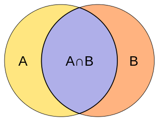
The Jaccard index, also known as the Jaccard similarity coefficient, is a statistic used for gauging the similarity and diversity of sample sets.
The Theil index is a statistic primarily used to measure economic inequality and other economic phenomena, though it has also been used to measure racial segregation.
The Atkinson index is a measure of income inequality developed by British economist Anthony Barnes Atkinson. The measure is useful in determining which end of the distribution contributed most to the observed inequality.
The mean absolute difference (univariate) is a measure of statistical dispersion equal to the average absolute difference of two independent values drawn from a probability distribution. A related statistic is the relative mean absolute difference, which is the mean absolute difference divided by the arithmetic mean, and equal to twice the Gini coefficient. The mean absolute difference is also known as the absolute mean difference and the Gini mean difference (GMD). The mean absolute difference is sometimes denoted by Δ or as MD.
In statistics, the generalized Pareto distribution (GPD) is a family of continuous probability distributions. It is often used to model the tails of another distribution. It is specified by three parameters: location , scale , and shape . Sometimes it is specified by only scale and shape and sometimes only by its shape parameter. Some references give the shape parameter as .

In probability and statistics, the log-logistic distribution is a continuous probability distribution for a non-negative random variable. It is used in survival analysis as a parametric model for events whose rate increases initially and decreases later, as, for example, mortality rate from cancer following diagnosis or treatment. It has also been used in hydrology to model stream flow and precipitation, in economics as a simple model of the distribution of wealth or income, and in networking to model the transmission times of data considering both the network and the software.
The Lorenz asymmetry coefficient (LAC) is a summary statistic of the Lorenz curve that measures the degree of asymmetry of the curve. The Lorenz curve is used to describe the inequality in the distribution of a quantity. The most common summary statistic for the Lorenz curve is the Gini coefficient, which is an overall measure of inequality within the population. The Lorenz asymmetry coefficient can be a useful supplement to the Gini coefficient. The Lorenz asymmetry coefficient is defined as

The Dagum distribution is a continuous probability distribution defined over positive real numbers. It is named after Camilo Dagum, who proposed it in a series of papers in the 1970s. The Dagum distribution arose from several variants of a new model on the size distribution of personal income and is mostly associated with the study of income distribution. There is both a three-parameter specification and a four-parameter specification of the Dagum distribution; a summary of the genesis of this distribution can be found in "A Guide to the Dagum Distributions". A general source on statistical size distributions often cited in work using the Dagum distribution is Statistical Size Distributions in Economics and Actuarial Sciences.

In probability theory and statistics, the Hermite distribution, named after Charles Hermite, is a discrete probability distribution used to model count data with more than one parameter. This distribution is flexible in terms of its ability to allow a moderate over-dispersion in the data.