In mathematics, the Newton polygon is a tool for understanding the behaviour of polynomials over local fields, or more generally, over ultrametric fields. In the original case, the ultrametric field of interest was essentially the field of formal Laurent series in the indeterminate X, i.e. the field of fractions of the formal power series ring , over , where was the real number or complex number field. This is still of considerable utility with respect to Puiseux expansions. The Newton polygon is an effective device for understanding the leading terms of the power series expansion solutions to equations where is a polynomial with coefficients in , the polynomial ring; that is, implicitly definedalgebraic functions. The exponents here are certain rational numbers, depending on the branch chosen; and the solutions themselves are power series in with for a denominator corresponding to the branch. The Newton polygon gives an effective, algorithmic approach to calculating .
After the introduction of the p-adic numbers, it was shown that the Newton polygon is just as useful in questions of ramification for local fields, and hence in algebraic number theory. Newton polygons have also been useful in the study of elliptic curves.
Definition
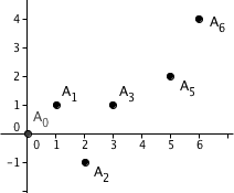
Construction of the Newton polygon of the polynomial 1 + 5 X + 1/5 X + 35 X + 25 X + 625 X with respect to the 5-adic valuation.
A priori, given a polynomial over a field, the behaviour of the roots (assuming it has roots) will be unknown. Newton polygons provide one technique for the study of the behaviour of the roots.
Let be a field endowed with a non-archimedean valuation, and let
with . Then the Newton polygon of is defined to be the lower boundary of the convex hull of the set of points ignoring the points with .
Restated geometrically, plot all of these points Pi on the xy-plane. Let's assume that the points indices increase from left to right (P0 is the leftmost point, Pn is the rightmost point). Then, starting at P0, draw a ray straight down parallel with the y-axis, and rotate this ray counter-clockwise until it hits the point Pk1 (not necessarily P1). Break the ray here. Now draw a second ray from Pk1 straight down parallel with the y-axis, and rotate this ray counter-clockwise until it hits the point Pk2. Continue until the process reaches the point Pn; the resulting polygon (containing the points P0, Pk1, Pk2, ..., Pkm, Pn) is the Newton polygon.
Another, perhaps more intuitive way to view this process is this: consider a rubber band surrounding all the points P0, ..., Pn. Stretch the band upwards, such that the band is stuck on its lower side by some of the points (the points act like nails, partially hammered into the xy plane). The vertices of the Newton polygon are exactly those points.
For a neat diagram of this see Ch6 §3 of "Local Fields" by JWS Cassels, LMS Student Texts 3, CUP 1986. It is on p99 of the 1986 paperback edition.
Main theorem
With the notations in the previous section, the main result concerning the Newton polygon is the following theorem,[1] which states that the valuation of the roots of are entirely determined by its Newton polygon:
Let be the slopes of the line segments of the Newton polygon of (as defined above) arranged in increasing order, and let be the corresponding lengths of the line segments projected onto the x-axis (i.e. if we have a line segment stretching between the points and then the length is ).
The are distinct;
;
if is a root of in , ;
for every , the number of roots of whose valuations are equal to (counting multiplicities) is at most , with equality if splits into the product of linear factors over .
Corollaries and applications
With the notation of the previous sections, we denote, in what follows, by the splitting field of over , and by an extension of to .
Newton polygon theorem is often used to show the irreducibility of polynomials, as in the next corollary for example:
Suppose that the valuation is discrete and normalized, and that the Newton polynomial of contains only one segment whose slope is and projection on the x-axis is . If , with coprime to , then is irreducible over . In particular, since the Newton polygon of an Eisenstein polynomial consists of a single segment of slope connecting and , Eisenstein criterion follows.
Indeed, by the main theorem, if is a root of , If were not irreducible over , then the degree of would be , and there would hold . But this is impossible since with coprime to .
Another simple corollary is the following:
Assume that is Henselian. If the Newton polygon of fulfills for some , then has a root in .
Proof: By the main theorem, must have a single root whose valuation is In particular, is separable over . If does not belong to , has a distinct Galois conjugate over , with ,[2] and is a root of , a contradiction.
More generally, the following factorization theorem holds:
Assume that is Henselian. Then , where , is monic for every , the roots of are of valuation , and .[3]
Moreover, , and if is coprime to , is irreducible over .
Proof: For every , denote by the product of the monomials such that is a root of and . We also denote the factorization of in into prime monic factors Let be a root of . We can assume that is the minimal polynomial of over . If is a root of , there exists a K-automorphism of that sends to , and we have since is Henselian. Therefore is also a root of . Moreover, every root of of multiplicity is clearly a root of of multiplicity , since repeated roots share obviously the same valuation. This shows that divides Let . Choose a root of . Notice that the roots of are distinct from the roots of . Repeat the previous argument with the minimal polynomial of over , assumed w.l.g. to be , to show that divides . Continuing this process until all the roots of are exhausted, one eventually arrives to , with . This shows that , monic. But the are coprime since their roots have distinct valuations. Hence clearly , showing the main contention. The fact that follows from the main theorem, and so does the fact that , by remarking that the Newton polygon of can have only one segment joining to . The condition for the irreducibility of follows from the corollary above. (q.e.d.)
The following is an immediate corollary of the factorization above, and constitutes a test for the reducibility of polynomials over Henselian fields:
Assume that is Henselian. If the Newton polygon does not reduce to a single segment then is reducible over .
Other applications of the Newton polygon comes from the fact that a Newton Polygon is sometimes a special case of a Newton polytope, and can be used to construct asymptotic solutions of two-variable polynomial equations like
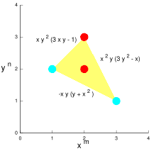
This diagram shows the Newton polygon for P(x,y) = 3xy − xy + 2xy − xy, with positive monomials in red and negative monomials in cyan. Faces are labelled with the limiting terms they correspond to.
Newton polygons are named after Isaac Newton, who first described them and some of their uses in correspondence from the year 1676 addressed to Henry Oldenburg.[4]
In the mathematical field of representation theory, a weight of an algebra A over a field F is an algebra homomorphism from A to F, or equivalently, a one-dimensional representation of A over F. It is the algebra analogue of a multiplicative character of a group. The importance of the concept, however, stems from its application to representations of Lie algebras and hence also to representations of algebraic and Lie groups. In this context, a weight of a representation is a generalization of the notion of an eigenvalue, and the corresponding eigenspace is called a weight space.
In mathematics, the classical orthogonal polynomials are the most widely used orthogonal polynomials: the Hermite polynomials, Laguerre polynomials, Jacobi polynomials.
In mathematics and theoretical physics, the term quantum group denotes one of a few different kinds of noncommutative algebras with additional structure. These include Drinfeld–Jimbo type quantum groups, compact matrix quantum groups, and bicrossproduct quantum groups. Despite their name, they do not themselves have a natural group structure, though they are in some sense 'close' to a group.
In linear algebra, the Frobenius companion matrix of the monic polynomial is the square matrix defined as
In mathematics, a Lie algebra is semisimple if it is a direct sum of simple Lie algebras.
Interior-point methods are algorithms for solving linear and non-linear convex optimization problems. IPMs combine two advantages of previously-known algorithms:
Verma modules, named after Daya-Nand Verma, are objects in the representation theory of Lie algebras, a branch of mathematics.
In mathematics, Schur polynomials, named after Issai Schur, are certain symmetric polynomials in n variables, indexed by partitions, that generalize the elementary symmetric polynomials and the complete homogeneous symmetric polynomials. In representation theory they are the characters of polynomial irreducible representations of the general linear groups. The Schur polynomials form a linear basis for the space of all symmetric polynomials. Any product of Schur polynomials can be written as a linear combination of Schur polynomials with non-negative integral coefficients; the values of these coefficients is given combinatorially by the Littlewood–Richardson rule. More generally, skew Schur polynomials are associated with pairs of partitions and have similar properties to Schur polynomials.
In mathematics, Hua's lemma, named for Hua Loo-keng, is an estimate for exponential sums.
In probability theory, the inverse Gaussian distribution is a two-parameter family of continuous probability distributions with support on (0,∞).
In mathematics, the Jack function is a generalization of the Jack polynomial, introduced by Henry Jack. The Jack polynomial is a homogeneous, symmetric polynomial which generalizes the Schur and zonal polynomials, and is in turn generalized by the Heckman–Opdam polynomials and Macdonald polynomials.
A ratio distribution is a probability distribution constructed as the distribution of the ratio of random variables having two other known distributions. Given two random variables X and Y, the distribution of the random variable Z that is formed as the ratio Z = X/Y is a ratio distribution.
In mathematics, Macdonald polynomialsPλ(x; t,q) are a family of orthogonal symmetric polynomials in several variables, introduced by Macdonald in 1987. He later introduced a non-symmetric generalization in 1995. Macdonald originally associated his polynomials with weights λ of finite root systems and used just one variable t, but later realized that it is more natural to associate them with affine root systems rather than finite root systems, in which case the variable t can be replaced by several different variables t=(t1,...,tk), one for each of the k orbits of roots in the affine root system. The Macdonald polynomials are polynomials in n variables x=(x1,...,xn), where n is the rank of the affine root system. They generalize many other families of orthogonal polynomials, such as Jack polynomials and Hall–Littlewood polynomials and Askey–Wilson polynomials, which in turn include most of the named 1-variable orthogonal polynomials as special cases. Koornwinder polynomials are Macdonald polynomials of certain non-reduced root systems. They have deep relationships with affine Hecke algebras and Hilbert schemes, which were used to prove several conjectures made by Macdonald about them.
The Jenkins–Traub algorithm for polynomial zeros is a fast globally convergent iterative polynomial root-finding method published in 1970 by Michael A. Jenkins and Joseph F. Traub. They gave two variants, one for general polynomials with complex coefficients, commonly known as the "CPOLY" algorithm, and a more complicated variant for the special case of polynomials with real coefficients, commonly known as the "RPOLY" algorithm. The latter is "practically a standard in black-box polynomial root-finders".
In probability theory and statistics, the normal-inverse-gamma distribution is a four-parameter family of multivariate continuous probability distributions. It is the conjugate prior of a normal distribution with unknown mean and variance.
In mathematics, the Kostka number is a non-negative integer that is equal to the number of semistandard Young tableaux of shape and weight . They were introduced by the mathematician Carl Kostka in his study of symmetric functions.
In probability theory and statistics, the Poisson distribution is a discrete probability distribution that expresses the probability of a given number of events occurring in a fixed interval of time if these events occur with a known constant mean rate and independently of the time since the last event. It can also be used for the number of events in other types of intervals than time, and in dimension greater than 1.
A geometric stable distribution or geo-stable distribution is a type of leptokurtic probability distribution. Geometric stable distributions were introduced in Klebanov, L. B., Maniya, G. M., and Melamed, I. A. (1985). A problem of Zolotarev and analogs of infinitely divisible and stable distributions in a scheme for summing a random number of random variables. These distributions are analogues for stable distributions for the case when the number of summands is random, independent of the distribution of summand, and having geometric distribution. The geometric stable distribution may be symmetric or asymmetric. A symmetric geometric stable distribution is also referred to as a Linnik distribution. The Laplace distribution and asymmetric Laplace distribution are special cases of the geometric stable distribution. The Mittag-Leffler distribution is also a special case of a geometric stable distribution.
In theoretical physics, relativistic Lagrangian mechanics is Lagrangian mechanics applied in the context of special relativity and general relativity.
In the theory of Lie groups, Lie algebras and their representation theory, a Lie algebra extensione is an enlargement of a given Lie algebra g by another Lie algebra h. Extensions arise in several ways. There is the trivial extension obtained by taking a direct sum of two Lie algebras. Other types are the split extension and the central extension. Extensions may arise naturally, for instance, when forming a Lie algebra from projective group representations. Such a Lie algebra will contain central charges.
References
↑ For an interesting demonstration based on hyperfields, see Matthew Baker, Oliver Lorscheid, (2021). Descartes' rule of signs, Newton polygons, and polynomials over hyperfields.Journal of Algebra, Volume 569, p. 416-441.
↑ Recall that in Henselian rings, any valuation extends uniquely to every algebraic extension of the base field. Hence extends uniquely to . But is an extension of for every automorphism of , therefore
↑ J. W. S. Cassels, Local Fields, Chap. 6, thm. 3.1.
This page is based on this Wikipedia article Text is available under the CC BY-SA 4.0 license; additional terms may apply. Images, videos and audio are available under their respective licenses.