In computing, a hash table, also known as a hash map or a hash set, is a data structure that implements an associative array, also called a dictionary, which is an abstract data type that maps keys to values. A hash table uses a hash function to compute an index, also called a hash code, into an array of buckets or slots, from which the desired value can be found. During lookup, the key is hashed and the resulting hash indicates where the corresponding value is stored.

In computer science, a heap is a tree-based data structure that satisfies the heap property: In a max heap, for any given node C, if P is a parent node of C, then the key of P is greater than or equal to the key of C. In a min heap, the key of P is less than or equal to the key of C. The node at the "top" of the heap is called the root node.
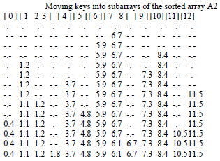
Insertion sort is a simple sorting algorithm that builds the final sorted array (or list) one item at a time by comparisons. It is much less efficient on large lists than more advanced algorithms such as quicksort, heapsort, or merge sort. However, insertion sort provides several advantages:
In computer science, merge sort is an efficient, general-purpose, and comparison-based sorting algorithm. Most implementations produce a stable sort, which means that the relative order of equal elements is the same in the input and output. Merge sort is a divide-and-conquer algorithm that was invented by John von Neumann in 1945. A detailed description and analysis of bottom-up merge sort appeared in a report by Goldstine and von Neumann as early as 1948.
In computer science, radix sort is a non-comparative sorting algorithm. It avoids comparison by creating and distributing elements into buckets according to their radix. For elements with more than one significant digit, this bucketing process is repeated for each digit, while preserving the ordering of the prior step, until all digits have been considered. For this reason, radix sort has also been called bucket sort and digital sort.
In computer science, a sorting algorithm is an algorithm that puts elements of a list into an order. The most frequently used orders are numerical order and lexicographical order, and either ascending or descending. Efficient sorting is important for optimizing the efficiency of other algorithms that require input data to be in sorted lists. Sorting is also often useful for canonicalizing data and for producing human-readable output.

A binary heap is a heap data structure that takes the form of a binary tree. Binary heaps are a common way of implementing priority queues. The binary heap was introduced by J. W. J. Williams in 1964, as a data structure for heapsort.

Shellsort, also known as Shell sort or Shell's method, is an in-place comparison sort. It can be seen as either a generalization of sorting by exchange or sorting by insertion. The method starts by sorting pairs of elements far apart from each other, then progressively reducing the gap between elements to be compared. By starting with far-apart elements, it can move some out-of-place elements into the position faster than a simple nearest-neighbor exchange. Donald Shell published the first version of this sort in 1959. The running time of Shellsort is heavily dependent on the gap sequence it uses. For many practical variants, determining their time complexity remains an open problem.

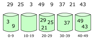
Bucket sort, or bin sort, is a sorting algorithm that works by distributing the elements of an array into a number of buckets. Each bucket is then sorted individually, either using a different sorting algorithm, or by recursively applying the bucket sorting algorithm. It is a distribution sort, a generalization of pigeonhole sort that allows multiple keys per bucket, and is a cousin of radix sort in the most-to-least significant digit flavor. Bucket sort can be implemented with comparisons and therefore can also be considered a comparison sort algorithm. The computational complexity depends on the algorithm used to sort each bucket, the number of buckets to use, and whether the input is uniformly distributed.
In computer science, counting sort is an algorithm for sorting a collection of objects according to keys that are small positive integers; that is, it is an integer sorting algorithm. It operates by counting the number of objects that possess distinct key values, and applying prefix sum on those counts to determine the positions of each key value in the output sequence. Its running time is linear in the number of items and the difference between the maximum key value and the minimum key value, so it is only suitable for direct use in situations where the variation in keys is not significantly greater than the number of items. It is often used as a subroutine in radix sort, another sorting algorithm, which can handle larger keys more efficiently.
A Bloom filter is a space-efficient probabilistic data structure, conceived by Burton Howard Bloom in 1970, that is used to test whether an element is a member of a set. False positive matches are possible, but false negatives are not – in other words, a query returns either "possibly in set" or "definitely not in set". Elements can be added to the set, but not removed ; the more items added, the larger the probability of false positives.
In computing, a persistent data structure or not ephemeral data structure is a data structure that always preserves the previous version of itself when it is modified. Such data structures are effectively immutable, as their operations do not (visibly) update the structure in-place, but instead always yield a new updated structure. The term was introduced in Driscoll, Sarnak, Sleator, and Tarjan's 1986 article.

Quicksort is an efficient, general-purpose sorting algorithm. Quicksort was developed by British computer scientist Tony Hoare in 1959 and published in 1961. It is still a commonly used algorithm for sorting. Overall, it is slightly faster than merge sort and heapsort for randomized data, particularly on larger distributions.
2-choice hashing, also known as 2-choice chaining, is "a variant of a hash table in which keys are added by hashing with two hash functions. The key is put in the array position with the fewer (colliding) keys. Some collision resolution scheme is needed, unless keys are kept in buckets. The average-case cost of a successful search is , where is the number of keys and is the size of the array. The most collisions is with high probability."
Database tables and indexes may be stored on disk in one of a number of forms, including ordered/unordered flat files, ISAM, heap files, hash buckets, or B+ trees. Each form has its own particular advantages and disadvantages. The most commonly used forms are B-trees and ISAM. Such forms or structures are one aspect of the overall schema used by a database engine to store information.
Flashsort is a distribution sorting algorithm showing linear computational complexity O(n) for uniformly distributed data sets and relatively little additional memory requirement. The original work was published in 1998 by Karl-Dietrich Neubert.
Samplesort is a sorting algorithm that is a divide and conquer algorithm often used in parallel processing systems. Conventional divide and conquer sorting algorithms partitions the array into sub-intervals or buckets. The buckets are then sorted individually and then concatenated together. However, if the array is non-uniformly distributed, the performance of these sorting algorithms can be significantly throttled. Samplesort addresses this issue by selecting a sample of size s from the n-element sequence, and determining the range of the buckets by sorting the sample and choosing p−1 < s elements from the result. These elements then divide the array into p approximately equal-sized buckets. Samplesort is described in the 1970 paper, "Samplesort: A Sampling Approach to Minimal Storage Tree Sorting", by W. D. Frazer and A. C. McKellar.
Block sort, or block merge sort, is a sorting algorithm combining at least two merge operations with an insertion sort to arrive at O(n log n) (see Big O notation) in-place stable sorting time. It gets its name from the observation that merging two sorted lists, A and B, is equivalent to breaking A into evenly sized blocks, inserting each A block into B under special rules, and merging AB pairs.
The cache-oblivious distribution sort is a comparison-based sorting algorithm. It is similar to quicksort, but it is a cache-oblivious algorithm, designed for a setting where the number of elements to sort is too large to fit in a cache where operations are done. In the external memory model, the number of memory transfers it needs to perform a sort of items on a machine with cache of size and cache lines of length is , under the tall cache assumption that . This number of memory transfers has been shown to be asymptotically optimal for comparison sorts. This distribution sort also achieves the asymptotically optimal runtime complexity of .
Interpolation sort is a sorting algorithm that is a kind of bucket sort. It uses an interpolation formula to assign data to the bucket. A general interpolation formula is: