Insertion sort

Insertion sort

Animation of insertion sort
Class	Sorting algorithm
Data structure	Array
Worst-case performance	${\displaystyle O(n^{2})}$ comparisons and swaps
Best-case performance	${\displaystyle O(n)}$ comparisons, ${\displaystyle O(1)}$ swaps
Average performance	${\displaystyle O(n^{2})}$ comparisons and swaps
Worst-case space complexity	${\displaystyle O(n)}$ total, ${\displaystyle O(1)}$ auxiliary
Optimal	No

Insertion sort is a simple sorting algorithm that builds the final sorted array (or list) one item at a time by comparisons. It is much less efficient on large lists than more advanced algorithms such as quicksort, heapsort, or merge sort. However, insertion sort provides several advantages:

• Simple implementation: Jon Bentley shows a three-line C/C++ version that is five lines when optimized. ^[1]
• Efficient for (quite) small data sets, much like other quadratic (i.e., O(n²)) sorting algorithms
• More efficient in practice than most other simple quadratic algorithms such as selection sort or bubble sort
• Adaptive, i.e., efficient for data sets that are already substantially sorted: the time complexity is O(kn) when each element in the input is no more than k places away from its sorted position
• Stable; i.e., does not change the relative order of elements with equal keys
• In-place; i.e., only requires a constant amount O(1) of additional memory space
• Online; i.e., can sort a list as it receives it

When people manually sort cards in a bridge hand, most use a method that is similar to insertion sort. ^[2]

Algorithm

A graphical example of insertion sort. The partial sorted list (black) initially contains only the first element in the list. With each iteration one element (red) is removed from the "not yet checked for order" input data and inserted in-place into the sorted list.

Insertion sort iterates, consuming one input element each repetition, and grows a sorted output list. At each iteration, insertion sort removes one element from the input data, finds the location it belongs within the sorted list, and inserts it there. It repeats until no input elements remain.

Sorting is typically done in-place, by iterating up the array, growing the sorted list behind it. At each array-position, it checks the value there against the largest value in the sorted list (which happens to be next to it, in the previous array-position checked). If larger, it leaves the element in place and moves to the next. If smaller, it finds the correct position within the sorted list, shifts all the larger values up to make a space, and inserts into that correct position.

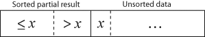
The resulting array after k iterations has the property where the first k + 1 entries are sorted ("+1" because the first entry is skipped). In each iteration the first remaining entry of the input is removed, and inserted into the result at the correct position, thus extending the result:

becomes

with each element greater than x copied to the right as it is compared against x.

The most common variant of insertion sort, which operates on arrays, can be described as follows:

1. Suppose there exists a function called Insert designed to insert a value into a sorted sequence at the beginning of an array. It operates by beginning at the end of the sequence and shifting each element one place to the right until a suitable position is found for the new element. The function has the side effect of overwriting the value stored immediately after the sorted sequence in the array.
2. To perform an insertion sort, begin at the left-most element of the array and invoke Insert to insert each element encountered into its correct position. The ordered sequence into which the element is inserted is stored at the beginning of the array in the set of indices already examined. Each insertion overwrites a single value: the value being inserted.

Pseudocode of the complete algorithm follows, where the arrays are zero-based: ^[1]

i ← 1 while i < length(A)     j ← i     while j > 0 and A[j-1] > A[j]         swap A[j] and A[j-1]         j ← j - 1     end while     i ← i + 1 end while

The outer loop runs over all the elements except the first one, because the single-element prefix A[0:1] is trivially sorted, so the invariant that the first i entries are sorted is true from the start. The inner loop moves element A[i] to its correct place so that after the loop, the first i+1 elements are sorted. Note that the and-operator in the test must use short-circuit evaluation, otherwise the test might result in an array bounds error, when j=0 and it tries to evaluate A[j-1] > A[j] (i.e. accessing A[-1] fails).

After expanding the swap operation in-place as x ← A[j]; A[j] ← A[j-1]; A[j-1] ← x (where x is a temporary variable), a slightly faster version can be produced that moves A[i] to its position in one go and only performs one assignment in the inner loop body: ^[1]

i ← 1 while i < length(A)     x ← A[i]     j ← i     while j > 0 and A[j-1] > x         A[j] ← A[j-1]         j ← j - 1     end while     A[j] ← x [3]      i ← i + 1 end while

The new inner loop shifts elements to the right to clear a spot for x = A[i].

The algorithm can also be implemented in a recursive way. The recursion just replaces the outer loop, calling itself and storing successively smaller values of n on the stack until n equals 0, where the function then returns up the call chain to execute the code after each recursive call starting with n equal to 1, with n increasing by 1 as each instance of the function returns to the prior instance. The initial call would be insertionSortR(A, length(A)-1).

function insertionSortR(array A, int n)     if n > 0         insertionSortR(A, n-1)         x ← A[n]         j ← n-1         while j >= 0 and A[j] > x             A[j+1] ← A[j]             j ← j-1         end while         A[j+1] ← x     end ifend function

It does not make the code any shorter, it also does not reduce the execution time, but it increases the additional memory consumption from O(1) to O(N) (at the deepest level of recursion the stack contains N references to the A array, each with accompanying value of variable n from N down to 1).

Best, worst, and average cases

The best case input is an array that is already sorted. In this case insertion sort has a linear running time (i.e., O(n)). During each iteration, the first remaining element of the input is only compared with the right-most element of the sorted subsection of the array.

The simplest worst case input is an array sorted in reverse order. The set of all worst case inputs consists of all arrays where each element is the smallest or second-smallest of the elements before it. In these cases every iteration of the inner loop will scan and shift the entire sorted subsection of the array before inserting the next element. This gives insertion sort a quadratic running time (i.e., O(n²)).

The average case is also quadratic, ^[4] which makes insertion sort impractical for sorting large arrays. However, insertion sort is one of the fastest algorithms for sorting very small arrays, even faster than quicksort; indeed, good quicksort implementations use insertion sort for arrays smaller than a certain threshold, also when arising as subproblems; the exact threshold must be determined experimentally and depends on the machine, but is commonly around ten.

Example: The following table shows the steps for sorting the sequence {3, 7, 4, 9, 5, 2, 6, 1}. In each step, the key under consideration is underlined. The key that was moved (or left in place because it was the biggest yet considered) in the previous step is marked with an asterisk.

3  7  4  9  5  2  6  1 3* 7  4  9  5  2  6  1 3  7* 4  9  5  2  6  1 3  4* 7  9  5  2  6  1 3  4  7  9* 5  2  6  1 3  4  5* 7  9  2  6  1 2* 3  4  5  7  9  6  1 2  3  4  5  6* 7  9  1 1* 2  3  4  5  6  7  9

Relation to other sorting algorithms

Insertion sort is very similar to selection sort. As in selection sort, after k passes through the array, the first k elements are in sorted order. However, the fundamental difference between the two algorithms is that insertion sort scans backwards from the current key, while selection sort scans forwards. This results in selection sort making the first k elements the k smallest elements of the unsorted input, while in insertion sort they are simply the first k elements of the input.

The primary advantage of insertion sort over selection sort is that selection sort must always scan all remaining elements to find the absolute smallest element in the unsorted portion of the list, while insertion sort requires only a single comparison when the (k + 1)-st element is greater than the k-th element; when this is frequently true (such as if the input array is already sorted or partially sorted), insertion sort is distinctly more efficient compared to selection sort. On average (assuming the rank of the (k + 1)-st element rank is random), insertion sort will require comparing and shifting half of the previous k elements, meaning that insertion sort will perform about half as many comparisons as selection sort on average.

In the worst case for insertion sort (when the input array is reverse-sorted), insertion sort performs just as many comparisons as selection sort. However, a disadvantage of insertion sort over selection sort is that it requires more writes due to the fact that, on each iteration, inserting the (k + 1)-st element into the sorted portion of the array requires many element swaps to shift all of the following elements, while only a single swap is required for each iteration of selection sort. In general, insertion sort will write to the array O(n²) times, whereas selection sort will write only O(n) times. For this reason selection sort may be preferable in cases where writing to memory is significantly more expensive than reading, such as with EEPROM or flash memory.

While some divide-and-conquer algorithms such as quicksort and mergesort outperform insertion sort for larger arrays, non-recursive sorting algorithms such as insertion sort or selection sort are generally faster for very small arrays (the exact size varies by environment and implementation, but is typically between 7 and 50 elements). Therefore, a useful optimization in the implementation of those algorithms is a hybrid approach, using the simpler algorithm when the array has been divided to a small size. ^[1]

Variants

D.L. Shell made substantial improvements to the algorithm; the modified version is called Shell sort. The sorting algorithm compares elements separated by a distance that decreases on each pass. Shell sort has distinctly improved running times in practical work, with two simple variants requiring O(n^3/2) and O(n^4/3) running time. ^{[5] [6]}

If the cost of comparisons exceeds the cost of swaps, as is the case for example with string keys stored by reference or with human interaction (such as choosing one of a pair displayed side-by-side), then using binary insertion sort may yield better performance. ^[7] Binary insertion sort employs a binary search to determine the correct location to insert new elements, and therefore performs ⌈log₂ n⌉ comparisons in the worst case. When each element in the array is searched for and inserted this is O(n log n). ^[7] The algorithm as a whole still has a running time of O(n²) on average because of the series of swaps required for each insertion. ^[7]

The number of swaps can be reduced by calculating the position of multiple elements before moving them. For example, if the target position of two elements is calculated before they are moved into the proper position, the number of swaps can be reduced by about 25% for random data. In the extreme case, this variant works similar to merge sort.

A variant named binary merge sort uses a binary insertion sort to sort groups of 32 elements, followed by a final sort using merge sort. It combines the speed of insertion sort on small data sets with the speed of merge sort on large data sets. ^[8]

To avoid having to make a series of swaps for each insertion, the input could be stored in a linked list, which allows elements to be spliced into or out of the list in constant time when the position in the list is known. However, searching a linked list requires sequentially following the links to the desired position: a linked list does not have random access, so it cannot use a faster method such as binary search. Therefore, the running time required for searching is O(n), and the time for sorting is O(n²). If a more sophisticated data structure (e.g., heap or binary tree) is used, the time required for searching and insertion can be reduced significantly; this is the essence of heap sort and binary tree sort.

In 2006 Bender, Martin Farach-Colton, and Mosteiro published a new variant of insertion sort called library sort or gapped insertion sort that leaves a small number of unused spaces (i.e., "gaps") spread throughout the array. The benefit is that insertions need only shift elements over until a gap is reached. The authors show that this sorting algorithm runs with high probability in O(n log n) time. ^[9]

If a skip list is used, the insertion time is brought down to O(log n), and swaps are not needed because the skip list is implemented on a linked list structure. The final running time for insertion would be O(n log n).

List insertion sort code in C

If the items are stored in a linked list, then the list can be sorted with O(1) additional space. The algorithm starts with an initially empty (and therefore trivially sorted) list. The input items are taken off the list one at a time, and then inserted in the proper place in the sorted list. When the input list is empty, the sorted list has the desired result.

structLIST*SortList1(structLIST*pList){// zero or one element in listif(pList==NULL||pList->pNext==NULL)returnpList;// head is the first element of resulting sorted liststructLIST*head=NULL;while(pList!=NULL){structLIST*current=pList;pList=pList->pNext;if(head==NULL||current->iValue<head->iValue){// insert into the head of the sorted list// or as the first element into an empty sorted listcurrent->pNext=head;head=current;}else{// insert current element into proper position in non-empty sorted liststructLIST*p=head;while(p!=NULL){if(p->pNext==NULL||// last element of the sorted listcurrent->iValue<p->pNext->iValue)// middle of the list{// insert into middle of the sorted list or as the last elementcurrent->pNext=p->pNext;p->pNext=current;break;// done}p=p->pNext;}}}returnhead;}

The algorithm below uses a trailing pointer ^[10] for the insertion into the sorted list. A simpler recursive method rebuilds the list each time (rather than splicing) and can use O(n) stack space.

structLIST{structLIST*pNext;intiValue;};structLIST*SortList(structLIST*pList){// zero or one element in listif(!pList||!pList->pNext)returnpList;/* build up the sorted array from the empty list */structLIST*pSorted=NULL;/* take items off the input list one by one until empty */while(pList!=NULL){/* remember the head */structLIST*pHead=pList;/* trailing pointer for efficient splice */structLIST**ppTrail=&pSorted;/* pop head off list */pList=pList->pNext;/* splice head into sorted list at proper place */while(!(*ppTrail==NULL||pHead->iValue<(*ppTrail)->iValue)){/* does head belong here? *//* no - continue down the list */ppTrail=&(*ppTrail)->pNext;}pHead->pNext=*ppTrail;*ppTrail=pHead;}returnpSorted;}

References

1. Bentley, Jon (2000). "Column 11: Sorting". Programming Pearls (2nd ed.). ACM Press / Addison-Wesley. pp. 115–116. ISBN   978-0-201-65788-3. OCLC   1047840657.
2. Sedgewick, Robert (1983). Algorithms . Addison-Wesley. p. 95. ISBN   978-0-201-06672-2.
3. Cormen, Thomas H.; Leiserson, Charles E.; Rivest, Ronald L.; Stein, Clifford (2009) [1990], "Section 2.1: Insertion sort", Introduction to Algorithms (3rd ed.), MIT Press and McGraw-Hill, pp. 16–18, ISBN   0-262-03384-4 . See in particular p. 18.
4. Schwarz, Keith. "Why is insertion sort Θ(n^2) in the average case? (answer by "templatetypedef")". Stack Overflow.
5. Frank, R. M.; Lazarus, R. B. (1960). "A High-Speed Sorting Procedure". Communications of the ACM. 3 (1): 20–22. doi: 10.1145/366947.366957 . S2CID   34066017.
6. Sedgewick, Robert (1986). "A New Upper Bound for Shellsort". Journal of Algorithms. 7 (2): 159–173. doi:10.1016/0196-6774(86)90001-5.
7. Samanta, Debasis (2008). Classic Data Structures. PHI Learning. p. 549. ISBN   9788120337312.
8. "Binary Merge Sort"
9. Bender, Michael A.; Farach-Colton, Martín; Mosteiro, Miguel A. (2006), "Insertion sort is O(n log n)", Theory of Computing Systems, 39 (3): 391–397, arXiv: cs/0407003 , doi:10.1007/s00224-005-1237-z, MR   2218409, S2CID   14701669
10. Hill, Curt (ed.), "Trailing Pointer Technique", Euler, Valley City State University, archived from the original on 26 April 2012, retrieved 22 September 2012.

Further reading

• Knuth, Donald (1998), "5.2.1: Sorting by Insertion", The Art of Computer Programming , vol. 3. Sorting and Searching (second ed.), Addison-Wesley, pp. 80–105, ISBN   0-201-89685-0 .

External links

• Animated Sorting Algorithms: Insertion Sort at the Wayback Machine (archived 8 March 2015) – graphical demonstration
• Adamovsky, John Paul, Binary Insertion Sort – Scoreboard – Complete Investigation and C Implementation, Pathcom.
• Insertion Sort – a comparison with other O(n²) sorting algorithms, UK: Core war.
• Insertion sort (C) (wiki), LiteratePrograms – implementations of insertion sort in C and several other programming languages