"Sinc" redirects here. For the designation used in the United Kingdom for areas of wildlife interest, see Site of Importance for Nature Conservation. For the signal processing filter based on this function, see Sinc filter.
In either case, the value at x = 0 is defined to be the limiting value
for all real a ≠ 0 (the limit can be proven using the squeeze theorem).
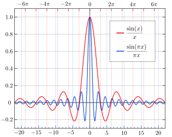
The normalization causes the definite integral of the function over the real numbers to equal 1 (whereas the same integral of the unnormalized sinc function has a value of π). As a further useful property, the zeros of the normalized sinc function are the nonzero integer values of x.
The only difference between the two definitions is in the scaling of the independent variable (the x axis) by a factor of π. In both cases, the value of the function at the removable singularity at zero is understood to be the limit value 1. The sinc function is then analytic everywhere and hence an entire function.
The function has also been called the cardinal sine or sine cardinal function.[3][4] The term sinc/ˈsɪŋk/ was introduced by Philip M.Woodward in his 1952 article "Information theory and inverse probability in telecommunication", in which he said that the function "occurs so often in Fourier analysis and its applications that it does seem to merit some notation of its own",[5] and his 1953 book Probability and Information Theory, with Applications to Radar.[6][7] The function itself was first mathematically derived in this form by Lord Rayleigh in his expression (Rayleigh's formula) for the zeroth-order spherical Bessel function of the first kind.
Properties
The local maxima and minima (small white dots) of the unnormalized, red sinc function correspond to its intersections with the blue cosine function.
The zero crossings of the unnormalized sinc are at non-zero integer multiples of π, while zero crossings of the normalized sinc occur at non-zero integers.
The local maxima and minima of the unnormalized sinc correspond to its intersections with the cosine function. That is, sin(ξ)/ξ = cos(ξ) for all points ξ where the derivative of sin(x)/x is zero and thus a local extremum is reached. This follows from the derivative of the sinc function:
The first few terms of the infinite series for the x coordinate of the n-th extremum with positive x coordinate are
where
and where odd n lead to a local minimum, and even n to a local maximum. Because of symmetry around the y axis, there exist extrema with x coordinates −xn. In addition, there is an absolute maximum at ξ0 = (0, 1).
The normalized sinc function has a simple representation as the infinite product:
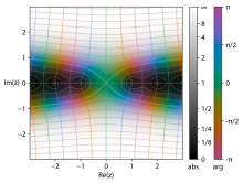
The cardinal sine function sinc(z) plotted in the complex plane from -2-2i to 2+2i
The normalized sinc function has properties that make it ideal in relationship to interpolation of sampledbandlimited functions:
It is an interpolating function, i.e., sinc(0) = 1, and sinc(k) = 0 for nonzero integerk.
The functions xk(t) = sinc(t − k) (k integer) form an orthonormal basis for bandlimited functions in the function spaceL2(R), with highest angular frequency ωH = π (that is, highest cycle frequency fH = 1/2).
Other properties of the two sinc functions include:
The unnormalized sinc is the zeroth-order spherical Bessel function of the first kind, j0(x). The normalized sinc is j0(πx).
This is not an ordinary limit, since the left side does not converge. Rather, it means that
for every Schwartz function, as can be seen from the Fourier inversion theorem. In the above expression, as a → 0, the number of oscillations per unit length of the sinc function approaches infinity. Nevertheless, the expression always oscillates inside an envelope of ±1/πx, regardless of the value of a.
This complicates the informal picture of δ(x) as being zero for all x except at the point x = 0, and illustrates the problem of thinking of the delta function as a function rather than as a distribution. A similar situation is found in the Gibbs phenomenon.
Summation
All sums in this section refer to the unnormalized sinc function.
The sum of sinc(n) over integer n from 1 to ∞ equals π − 1/2:
The sum of the squares also equals π − 1/2:[10][11]
When the signs of the addends alternate and begin with +, the sum equals 1/2:
The alternating sums of the squares and cubes also equal 1/2:[12]
Series expansion
The Taylor series of the unnormalized sinc function can be obtained from that of the sine (which also yields its value of 1 at x = 0):
The series converges for all x. The normalized version follows easily:
Euler famously compared this series to the expansion of the infinite product form to solve the Basel problem.
Higher dimensions
The product of 1-D sinc functions readily provides a multivariate sinc function for the square Cartesian grid (lattice): sincC(x, y) = sinc(x) sinc(y), whose Fourier transform is the indicator function of a square in the frequency space (i.e., the brick wall defined in 2-D space). The sinc function for a non-Cartesian lattice (e.g., hexagonal lattice) is a function whose Fourier transform is the indicator function of the Brillouin zone of that lattice. For example, the sinc function for the hexagonal lattice is a function whose Fourier transform is the indicator function of the unit hexagon in the frequency space. For a non-Cartesian lattice this function can not be obtained by a simple tensor product. However, the explicit formula for the sinc function for the hexagonal, body-centered cubic, face-centered cubic and other higher-dimensional lattices can be explicitly derived[13] using the geometric properties of Brillouin zones and their connection to zonotopes.
In physics, the cross section is a measure of the probability that a specific process will take place in a collision of two particles. For example, the Rutherford cross-section is a measure of probability that an alpha particle will be deflected by a given angle during an interaction with an atomic nucleus. Cross section is typically denoted σ (sigma) and is expressed in units of area, more specifically in barns. In a way, it can be thought of as the size of the object that the excitation must hit in order for the process to occur, but more exactly, it is a parameter of a stochastic process.
In mathematics, the trigonometric functions are real functions which relate an angle of a right-angled triangle to ratios of two side lengths. They are widely used in all sciences that are related to geometry, such as navigation, solid mechanics, celestial mechanics, geodesy, and many others. They are among the simplest periodic functions, and as such are also widely used for studying periodic phenomena through Fourier analysis.
In mathematics, an n-sphere or hypersphere is an n-dimensional generalization of the 1-dimensional circle and 2-dimensional sphere to any non-negative integer n. The n-sphere is the setting for n-dimensional spherical geometry.
The Navier–Stokes equations are partial differential equations which describe the motion of viscous fluid substances. They were named after French engineer and physicist Claude-Louis Navier and the Irish physicist and mathematician George Gabriel Stokes. They were developed over several decades of progressively building the theories, from 1822 (Navier) to 1842–1850 (Stokes).
In mathematics, Legendre polynomials, named after Adrien-Marie Legendre (1782), are a system of complete and orthogonal polynomials with a vast number of mathematical properties and numerous applications. They can be defined in many ways, and the various definitions highlight different aspects as well as suggest generalizations and connections to different mathematical structures and physical and numerical applications.
In mechanics and geometry, the 3D rotation group, often denoted SO(3), is the group of all rotations about the origin of three-dimensional Euclidean space under the operation of composition.
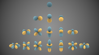
In mathematics and physical science, spherical harmonics are special functions defined on the surface of a sphere. They are often employed in solving partial differential equations in many scientific fields. A list of the spherical harmonics is available in Table of spherical harmonics.
In mathematics, the inverse trigonometric functions are the inverse functions of the trigonometric functions. Specifically, they are the inverses of the sine, cosine, tangent, cotangent, secant, and cosecant functions, and are used to obtain an angle from any of the angle's trigonometric ratios. Inverse trigonometric functions are widely used in engineering, navigation, physics, and geometry.
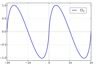
In mathematics, the Clausen function, introduced by Thomas Clausen, is a transcendental, special function of a single variable. It can variously be expressed in the form of a definite integral, a trigonometric series, and various other forms. It is intimately connected with the polylogarithm, inverse tangent integral, polygamma function, Riemann zeta function, Dirichlet eta function, and Dirichlet beta function.
This is a list of some vector calculus formulae for working with common curvilinear coordinate systems.
The rectangular function is defined as
Directional statistics is the subdiscipline of statistics that deals with directions, axes or rotations in Rn. More generally, directional statistics deals with observations on compact Riemannian manifolds including the Stiefel manifold.
In probability and statistics, a circular distribution or polar distribution is a probability distribution of a random variable whose values are angles, usually taken to be in the range [0, 2π). A circular distribution is often a continuous probability distribution, and hence has a probability density, but such distributions can also be discrete, in which case they are called circular lattice distributions. Circular distributions can be used even when the variables concerned are not explicitly angles: the main consideration is that there is not usually any real distinction between events occurring at the opposite ends of the range, and the division of the range could notionally be made at any point.
In mathematics, sine and cosine are trigonometric functions of an angle. The sine and cosine of an acute angle are defined in the context of a right triangle: for the specified angle, its sine is the ratio of the length of the side that is opposite that angle to the length of the longest side of the triangle, and the cosine is the ratio of the length of the adjacent leg to that of the hypotenuse. For an angle , the sine and cosine functions are denoted simply as and .
A pendulum is a body suspended from a fixed support so that it swings freely back and forth under the influence of gravity. When a pendulum is displaced sideways from its resting, equilibrium position, it is subject to a restoring force due to gravity that will accelerate it back towards the equilibrium position. When released, the restoring force acting on the pendulum's mass causes it to oscillate about the equilibrium position, swinging it back and forth. The mathematics of pendulums are in general quite complicated. Simplifying assumptions can be made, which in the case of a simple pendulum allow the equations of motion to be solved analytically for small-angle oscillations.
In mathematics, the axis–angle representation parameterizes a rotation in a three-dimensional Euclidean space by two quantities: a unit vector e indicating the direction (geometry) of an axis of rotation, and an angle of rotation θ describing the magnitude and sense of the rotation about the axis. Only two numbers, not three, are needed to define the direction of a unit vector e rooted at the origin because the magnitude of e is constrained. For example, the elevation and azimuth angles of e suffice to locate it in any particular Cartesian coordinate frame.
In fluid dynamics, the Oseen equations describe the flow of a viscous and incompressible fluid at small Reynolds numbers, as formulated by Carl Wilhelm Oseen in 1910. Oseen flow is an improved description of these flows, as compared to Stokes flow, with the (partial) inclusion of convective acceleration.
In optics, the Fraunhofer diffraction equation is used to model the diffraction of waves when the diffraction pattern is viewed at a long distance from the diffracting object, and also when it is viewed at the focal plane of an imaging lens.
This page is based on this Wikipedia article Text is available under the CC BY-SA 4.0 license; additional terms may apply. Images, videos and audio are available under their respective licenses.