Hamilton's principle

Last updated
As the system evolves, q traces a path through configuration space (only some are shown). The path taken by the system (red) has a stationary action (dS = 0) under small changes in the configuration of the system (dq). Least action principle.svg
As the system evolves, q traces a path through configuration space (only some are shown). The path taken by the system (red) has a stationary action (δS = 0) under small changes in the configuration of the system (δq).

In physics, Hamilton's principle is William Rowan Hamilton's formulation of the principle of stationary action. It states that the dynamics of a physical system are determined by a variational problem for a functional based on a single function, the Lagrangian, which may contain all physical information concerning the system and the forces acting on it. The variational problem is equivalent to and allows for the derivation of the differential equations of motion of the physical system. Although formulated originally for classical mechanics, Hamilton's principle also applies to classical fields such as the electromagnetic and gravitational fields, and plays an important role in quantum mechanics, quantum field theory and criticality theories.

Contents

Mathematical formulation

Hamilton's principle states that the true evolution q(t) of a system described by N generalized coordinates q = (q1, q2, ..., qN) between two specified states q1 = q(t1) and q2 = q(t2) at two specified times t1 and t2 is a stationary point (a point where the variation is zero) of the action functional

where is the Lagrangian function for the system. In other words, any first-order perturbation of the true evolution results in (at most) second-order changes in . The action is a functional, i.e., something that takes as its input a function and returns a single number, a scalar. In terms of functional analysis, Hamilton's principle states that the true evolution of a physical system is a solution of the functional equation

Hamilton's principle

That is, the system takes a path in configuration space for which the action is stationary, with fixed boundary conditions at the beginning and the end of the path.

Euler–Lagrange equations derived from the action integral

Requiring that the true trajectory q(t) be a stationary point of the action functional is equivalent to a set of differential equations for q(t) (the Euler–Lagrange equations), which may be derived as follows.

Let q(t) represent the true evolution of the system between two specified states q1 = q(t1) and q2 = q(t2) at two specified times t1 and t2, and let ε(t) be a small perturbation that is zero at the endpoints of the trajectory

To first order in the perturbation ε(t), the change in the action functional would be

where we have expanded the Lagrangian L to first order in the perturbation ε(t).

Applying integration by parts to the last term results in

The boundary conditions causes the first term to vanish

Hamilton's principle requires that this first-order change is zero for all possible perturbations ε(t), i.e., the true path is a stationary point of the action functional (either a minimum, maximum or saddle point). This requirement can be satisfied if and only if

Euler–Lagrange equations

These equations are called the Euler–Lagrange equations for the variational problem.

Canonical momenta and constants of motion

The conjugate momentumpk for a generalized coordinate qk is defined by the equation

An important special case of the Euler–Lagrange equation occurs when L does not contain a generalized coordinate qk explicitly,

that is, the conjugate momentum is a constant of the motion.

In such cases, the coordinate qk is called a cyclic coordinate. For example, if we use polar coordinates t, r, θ to describe the planar motion of a particle, and if L does not depend on θ, the conjugate momentum is the conserved angular momentum.

Example: Free particle in polar coordinates

Trivial examples help to appreciate the use of the action principle via the Euler–Lagrange equations. A free particle (mass m and velocity v) in Euclidean space moves in a straight line. Using the Euler–Lagrange equations, this can be shown in polar coordinates as follows. In the absence of a potential, the Lagrangian is simply equal to the kinetic energy

in orthonormal (x,y) coordinates, where the dot represents differentiation with respect to the curve parameter (usually the time, t). Therefore, upon application of the Euler–Lagrange equations,

And likewise for y. Thus the Euler–Lagrange formulation can be used to derive Newton's laws.

In polar coordinates (r, φ) the kinetic energy and hence the Lagrangian becomes

The radial r and φ components of the Euler–Lagrange equations become, respectively

remembering that r is also dependent on time and the product rule is needed to compute the total time derivative .

The solution of these two equations is given by

for a set of constants a, b, c, d determined by initial conditions. Thus, indeed, the solution is a straight line given in polar coordinates: a is the velocity, c is the distance of the closest approach to the origin, and d is the angle of motion.

Applied to deformable bodies

Hamilton's principle is an important variational principle in elastodynamics. As opposed to a system composed of rigid bodies, deformable bodies have an infinite number of degrees of freedom and occupy continuous regions of space; consequently, the state of the system is described by using continuous functions of space and time. The extended Hamilton Principle for such bodies is given by

where T is the kinetic energy, U is the elastic energy, We is the work done by external loads on the body, and t1, t2 the initial and final times. If the system is conservative, the work done by external forces may be derived from a scalar potential V. In this case,

This is called Hamilton's principle and it is invariant under coordinate transformations.

Comparison with Maupertuis' principle

Hamilton's principle and Maupertuis' principle are occasionally confused and both have been called the principle of least action. They differ in three important ways:

Action principle for fields

Classical field theory

The action principle can be extended to obtain the equations of motion for fields, such as the electromagnetic field or gravity.

The Einstein equation utilizes the Einstein–Hilbert action as constrained by a variational principle.

The path of a body in a gravitational field (i.e. free fall in space time, a so-called geodesic) can be found using the action principle.

Quantum mechanics and quantum field theory

In quantum mechanics, the system does not follow a single path whose action is stationary, but the behavior of the system depends on all imaginable paths and the value of their action. The action corresponding to the various paths is used to calculate the path integral, that gives the probability amplitudes of the various outcomes.

Although equivalent in classical mechanics with Newton's laws, the action principle is better suited for generalizations and plays an important role in modern physics. Indeed, this principle is one of the great generalizations in physical science. In particular, it is fully appreciated and best understood within quantum mechanics. Richard Feynman's path integral formulation of quantum mechanics is based on a stationary-action principle, using path integrals. Maxwell's equations can be derived as conditions of stationary action.

See also

Related Research Articles

<span class="mw-page-title-main">Equations of motion</span> Equations that describe the behavior of a physical system

In physics, equations of motion are equations that describe the behavior of a physical system in terms of its motion as a function of time. More specifically, the equations of motion describe the behavior of a physical system as a set of mathematical functions in terms of dynamic variables. These variables are usually spatial coordinates and time, but may include momentum components. The most general choice are generalized coordinates which can be any convenient variables characteristic of the physical system. The functions are defined in a Euclidean space in classical mechanics, but are replaced by curved spaces in relativity. If the dynamics of a system is known, the equations are the solutions for the differential equations describing the motion of the dynamics.

<span class="mw-page-title-main">Noether's theorem</span> Statement relating differentiable symmetries to conserved quantities

Noether's theorem or Noether's first theorem states that every differentiable symmetry of the action of a physical system with conservative forces has a corresponding conservation law. The theorem was proven by mathematician Emmy Noether in 1915 and published in 1918. The action of a physical system is the integral over time of a Lagrangian function, from which the system's behavior can be determined by the principle of least action. This theorem only applies to continuous and smooth symmetries over physical space.

<span class="mw-page-title-main">Fokker–Planck equation</span> Partial differential equation

In statistical mechanics and information theory, the Fokker–Planck equation is a partial differential equation that describes the time evolution of the probability density function of the velocity of a particle under the influence of drag forces and random forces, as in Brownian motion. The equation can be generalized to other observables as well. The Fokker-Planck equation has multiple applications in information theory, graph theory, data science, finance, economics etc.

The calculus of variations is a field of mathematical analysis that uses variations, which are small changes in functions and functionals, to find maxima and minima of functionals: mappings from a set of functions to the real numbers. Functionals are often expressed as definite integrals involving functions and their derivatives. Functions that maximize or minimize functionals may be found using the Euler–Lagrange equation of the calculus of variations.

<span class="mw-page-title-main">Hamiltonian mechanics</span> Formulation of classical mechanics using momenta

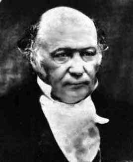
Hamiltonian mechanics emerged in 1833 as a reformulation of Lagrangian mechanics. Introduced by Sir William Rowan Hamilton, Hamiltonian mechanics replaces (generalized) velocities used in Lagrangian mechanics with (generalized) momenta. Both theories provide interpretations of classical mechanics and describe the same physical phenomena.

In the calculus of variations and classical mechanics, the Euler–Lagrange equations are a system of second-order ordinary differential equations whose solutions are stationary points of the given action functional. The equations were discovered in the 1750s by Swiss mathematician Leonhard Euler and Italian mathematician Joseph-Louis Lagrange.

In the calculus of variations, a field of mathematical analysis, the functional derivative relates a change in a functional to a change in a function on which the functional depends.

<span class="mw-page-title-main">Path integral formulation</span> Formulation of quantum mechanics

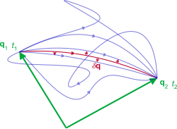
The path integral formulation is a description in quantum mechanics that generalizes the stationary action principle of classical mechanics. It replaces the classical notion of a single, unique classical trajectory for a system with a sum, or functional integral, over an infinity of quantum-mechanically possible trajectories to compute a quantum amplitude.

In theoretical physics and mathematical physics, analytical mechanics, or theoretical mechanics is a collection of closely related alternative formulations of classical mechanics. It was developed by many scientists and mathematicians during the 18th century and onward, after Newtonian mechanics. Since Newtonian mechanics considers vector quantities of motion, particularly accelerations, momenta, forces, of the constituents of the system, an alternative name for the mechanics governed by Newton's laws and Euler's laws is vectorial mechanics.

In Hamiltonian mechanics, a canonical transformation is a change of canonical coordinates (q, p, t) → that preserves the form of Hamilton's equations. This is sometimes known as form invariance. It need not preserve the form of the Hamiltonian itself. Canonical transformations are useful in their own right, and also form the basis for the Hamilton–Jacobi equations and Liouville's theorem.

In physics, particularly in quantum field theory, configurations of a physical system that satisfy classical equations of motion are called "on the mass shell" or simply more often on shell; while those that do not are called "off the mass shell", or off shell.

In physics, the Hamilton–Jacobi equation, named after William Rowan Hamilton and Carl Gustav Jacob Jacobi, is an alternative formulation of classical mechanics, equivalent to other formulations such as Newton's laws of motion, Lagrangian mechanics and Hamiltonian mechanics.

In mechanics, virtual work arises in the application of the principle of least action to the study of forces and movement of a mechanical system. The work of a force acting on a particle as it moves along a displacement is different for different displacements. Among all the possible displacements that a particle may follow, called virtual displacements, one will minimize the action. This displacement is therefore the displacement followed by the particle according to the principle of least action.

The work of a force on a particle along a virtual displacement is known as the virtual work.

A classical field theory is a physical theory that predicts how one or more physical fields interact with matter through field equations, without considering effects of quantization; theories that incorporate quantum mechanics are called quantum field theories. In most contexts, 'classical field theory' is specifically intended to describe electromagnetism and gravitation, two of the fundamental forces of nature.

<span class="mw-page-title-main">Liénard–Wiechert potential</span> Electromagnetic effect of point charges

The Liénard–Wiechert potentials describe the classical electromagnetic effect of a moving electric point charge in terms of a vector potential and a scalar potential in the Lorenz gauge. Stemming directly from Maxwell's equations, these describe the complete, relativistically correct, time-varying electromagnetic field for a point charge in arbitrary motion, but are not corrected for quantum mechanical effects. Electromagnetic radiation in the form of waves can be obtained from these potentials. These expressions were developed in part by Alfred-Marie Liénard in 1898 and independently by Emil Wiechert in 1900.

<span class="mw-page-title-main">Lagrangian mechanics</span> Formulation of classical mechanics

In physics, Lagrangian mechanics is a formulation of classical mechanics founded on the stationary-action principle. It was introduced by the Italian-French mathematician and astronomer Joseph-Louis Lagrange in his presentation to the Turin Academy of Science in 1760 culminating in his 1788 grand opus, Mécanique analytique.

In analytical mechanics and quantum field theory, minimal coupling refers to a coupling between fields which involves only the charge distribution and not higher multipole moments of the charge distribution. This minimal coupling is in contrast to, for example, Pauli coupling, which includes the magnetic moment of an electron directly in the Lagrangian.

<span class="mw-page-title-main">Relativistic Lagrangian mechanics</span> Mathematical formulation of special and general relativity

In theoretical physics, relativistic Lagrangian mechanics is Lagrangian mechanics applied in the context of special relativity and general relativity.

Lagrangian field theory is a formalism in classical field theory. It is the field-theoretic analogue of Lagrangian mechanics. Lagrangian mechanics is used to analyze the motion of a system of discrete particles each with a finite number of degrees of freedom. Lagrangian field theory applies to continua and fields, which have an infinite number of degrees of freedom.

Computational anatomy (CA) is the study of shape and form in medical imaging. The study of deformable shapes in computational anatomy rely on high-dimensional diffeomorphism groups which generate orbits of the form . In CA, this orbit is in general considered a smooth Riemannian manifold since at every point of the manifold there is an inner product inducing the norm on the tangent space that varies smoothly from point to point in the manifold of shapes . This is generated by viewing the group of diffeomorphisms as a Riemannian manifold with , associated to the tangent space at . This induces the norm and metric on the orbit under the action from the group of diffeomorphisms.

References

  1. R. Penrose (2007). The Road to Reality . Vintage books. p. 474. ISBN   978-0-679-77631-4.