In finance, the Sharpe ratio (also known as the Sharpe index, the Sharpe measure, and the reward-to-variability ratio) measures the performance of an investment such as a security or portfolio compared to a risk-free asset, after adjusting for its risk. It is defined as the difference between the returns of the investment and the risk-free return, divided by the standard deviation of the investment returns. It represents the additional amount of return that an investor receives per unit of increase in risk.
Since its revision by the original author, William Sharpe, in 1994,[2] the ex-ante Sharpe ratio is defined as:
where is the asset return, is the risk-free return (such as a U.S. Treasury security). is the expected value of the excess of the asset return over the benchmark return, and is the standard deviation of the asset excess return. The t-statistic will equal the Sharpe Ratio times the square root of T (the number of returns used for the calculation).
The ex-post Sharpe ratio uses the same equation as the one above but with realized returns of the asset and benchmark rather than expected returns; see the second example below.
The information ratio is a generalization of the Sharpe ratio that uses as benchmark some other, typically risky index rather than using risk-free returns.
Use in finance
The Sharpe ratio seeks to characterize how well the return of an asset compensates the investor for the risk taken. When comparing two assets, the one with a higher Sharpe ratio appears to provide better return for the same risk, which is usually attractive to investors.[3]
However, financial assets are often not normally distributed, so that standard deviation does not capture all aspects of risk. Ponzi schemes, for example, will have a high empirical Sharpe ratio until they fail. Similarly, a fund that sells low-strike put options will have a high empirical Sharpe ratio until one of those puts is exercised, creating a large loss. In both cases, the empirical standard deviation before failure gives no real indication of the size of the risk being run.[4]
Even in less extreme cases, a reliable empirical estimate of Sharpe ratio still requires the collection of return data over sufficient period for all aspects of the strategy returns to be observed. For example, data must be taken over decades if the algorithm sells an insurance that involves a high liability payout once every 5–10 years, and a high-frequency trading algorithm may only require a week of data if each trade occurs every 50 milliseconds, with care taken toward risk from unexpected but rare results that such testing did not capture (see flash crash).
Additionally, when examining the investment performance of assets with smoothing of returns (such as with-profits funds), the Sharpe ratio should be derived from the performance of the underlying assets rather than the fund returns (Such a model would invalidate the aforementioned Ponzi scheme, as desired).
Sharpe ratios, along with Treynor ratios and Jensen's alphas, are often used to rank the performance of portfolio or mutual fund managers. Berkshire Hathaway had a Sharpe ratio of 0.76 for the period 1976 to 2011, higher than any other stock or mutual fund with a history of more than 30 years. The stock market[specify] had a Sharpe ratio of 0.39 for the same period.[5]
Tests
Several statistical tests of the Sharpe ratio have been proposed. These include those proposed by Jobson & Korkie[6] and Gibbons, Ross & Shanken.[7]
History
In 1952, Arthur D. Roy suggested maximizing the ratio "(m-d)/σ", where m is expected gross return, d is some "disaster level" (a.k.a., minimum acceptable return, or MAR) and σ is standard deviation of returns.[8] This ratio is just the Sharpe ratio, only using minimum acceptable return instead of the risk-free rate in the numerator, and using standard deviation of returns instead of standard deviation of excess returns in the denominator. Roy's ratio is also related to the Sortino ratio, which also uses MAR in the numerator, but uses a different standard deviation (semi/downside deviation) in the denominator.
In 1966, William F. Sharpe developed what is now known as the Sharpe ratio.[1] Sharpe originally called it the "reward-to-variability" ratio before it began being called the Sharpe ratio by later academics and financial operators. The definition was:
Sharpe's 1994 revision acknowledged that the basis of comparison should be an applicable benchmark, which changes with time. After this revision, the definition is:
Note, if Rf is a constant risk-free return throughout the period,
The (original) Sharpe ratio has often been challenged with regard to its appropriateness as a fund performance measure during periods of declining markets.[9]
Examples
Example 1
Suppose the asset has an expected return of 15% in excess of the risk free rate. We typically do not know if the asset will have this return. We estimate the risk of the asset, defined as standard deviation of the asset's excess return, as 10%. The risk-free return is constant. Then the Sharpe ratio using the old definition is
Example 2
An investor has a portfolio with an expected return of 12% and a standard deviation of 10%. The rate of interest is 5%, and is risk-free.
The Sharpe ratio is:
Strengths and weaknesses
A negative Sharpe ratio means the portfolio has underperformed its benchmark. All other things being equal, an investor typically prefers a higher positive Sharpe ratio as it has either higher returns or lower volatility. However, a negative Sharpe ratio can be made higher by either increasing returns (a good thing) or increasing volatility (a bad thing). Thus, for negative values the Sharpe ratio does not correspond well to typical investor utility functions.
The Sharpe ratio is convenient because it can be calculated purely from any observed series of returns without need for additional information surrounding the source of profitability. However, this makes it vulnerable to manipulation if opportunities exist for smoothing or discretionary pricing of illiquid assets. Statistics such as the bias ratio and first order autocorrelation are sometimes used to indicate the potential presence of these problems.
While the Treynor ratio considers only the systematic risk of a portfolio, the Sharpe ratio considers both systematic and idiosyncratic risks. Which one is more relevant will depend on the portfolio context.
The returns measured can be of any frequency (i.e. daily, weekly, monthly or annually), as long as they are normally distributed, as the returns can always be annualized. Herein lies the underlying weakness of the ratio - asset returns are not normally distributed. Abnormalities like kurtosis, fatter tails and higher peaks, or skewness on the distribution can be problematic for the ratio, as standard deviation doesn't have the same effectiveness when these problems exist.[10]
For Brownian walk, Sharpe ratio is a dimensional quantity and has units , because the excess return and the volatility are proportional to and correspondingly. Kelly criterion is a dimensionless quantity, and, indeed, Kelly fraction is the numerical fraction of wealth suggested for the investment.
In some settings, the Kelly criterion can be used to convert the Sharpe ratio into a rate of return. The Kelly criterion gives the ideal size of the investment, which when adjusted by the period and expected rate of return per unit, gives a rate of return.[11]
The accuracy of Sharpe ratio estimators hinges on the statistical properties of returns, and these properties can vary considerably among strategies, portfolios, and over time.[12]
Drawback as fund selection criteria
Bailey and López de Prado (2012)[13] show that Sharpe ratios tend to be overstated in the case of hedge funds with short track records. These authors propose a probabilistic version of the Sharpe ratio that takes into account the asymmetry and fat-tails of the returns' distribution. With regards to the selection of portfolio managers on the basis of their Sharpe ratios, these authors have proposed a Sharpe ratio indifference curve[14] This curve illustrates the fact that it is efficient to hire portfolio managers with low and even negative Sharpe ratios, as long as their correlation to the other portfolio managers is sufficiently low.
Goetzmann, Ingersoll, Spiegel, and Welch (2002) determined that the best strategy to maximize a portfolio's Sharpe ratio, when both securities and options contracts on these securities are available for investment, is a portfolio of selling one out-of-the-money call and selling one out-of-the-money put. This portfolio generates an immediate positive payoff, has a large probability of generating modestly high returns, and has a small probability of generating huge losses. Shah (2014) observed that such a portfolio is not suitable for many investors, but fund sponsors who select fund managers primarily based on the Sharpe ratio will give incentives for fund managers to adopt such a strategy.[15]
In recent years, many financial websites have promoted the idea that a Sharpe Ratio "greater than 1 is considered acceptable; a ratio higher than 2.0 is considered very good; and a ratio above 3.0 is excellent." While it is unclear where this rubric originated online, it makes little sense since the magnitude of the Sharpe ratio is sensitive to the time period over which the underlying returns are measured. This is because the nominator of the ratio (returns) scales in proportion to time; while the denominator of the ratio (standard deviation) scales in proportion to the square root of time. Most diversified indexes of equities, bonds, mortgages or commodities have annualized Sharpe ratios below 1, which suggests that a Sharpe ratio consistently above 2.0 or 3.0 is unrealistic.
In statistics, the standard deviation is a measure of the amount of variation of a random variable expected about its mean. A low standard deviation indicates that the values tend to be close to the mean of the set, while a high standard deviation indicates that the values are spread out over a wider range.
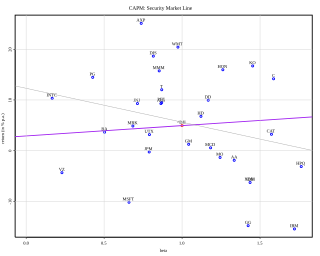
In finance, the capital asset pricing model (CAPM) is a model used to determine a theoretically appropriate required rate of return of an asset, to make decisions about adding assets to a well-diversified portfolio.
Modern portfolio theory (MPT), or mean-variance analysis, is a mathematical framework for assembling a portfolio of assets such that the expected return is maximized for a given level of risk. It is a formalization and extension of diversification in investing, the idea that owning different kinds of financial assets is less risky than owning only one type. Its key insight is that an asset's risk and return should not be assessed by itself, but by how it contributes to a portfolio's overall risk and return. The variance of return is used as a measure of risk, because it is tractable when assets are combined into portfolios. Often, the historical variance and covariance of returns is used as a proxy for the forward-looking versions of these quantities, but other, more sophisticated methods are available.
In finance, the beta is a statistic that measures the expected increase or decrease of an individual stock price in proportion to movements of the stock market as a whole. Beta can be used to indicate the contribution of an individual asset to the market risk of a portfolio when it is added in small quantity. It refers to an asset's non-diversifiable risk, systematic risk, or market risk. Beta is not a measure of idiosyncratic risk.
The Sortino ratio measures the risk-adjusted return of an investment asset, portfolio, or strategy. It is a modification of the Sharpe ratio but penalizes only those returns falling below a user-specified target or required rate of return, while the Sharpe ratio penalizes both upside and downside volatility equally. Though both ratios measure an investment's risk-adjusted return, they do so in significantly different ways that will frequently lead to differing conclusions as to the true nature of the investment's return-generating efficiency.
In finance, Jensen's alpha is used to determine the abnormal return of a security or portfolio of securities over the theoretical expected return. It is a version of the standard alpha based on a theoretical performance instead of a market index.
The Treynor reward to volatility model, named after Jack L. Treynor, is a measurement of the returns earned in excess of that which could have been earned on an investment that has no diversifiable risk, per unit of market risk assumed.
The upside-potential ratio is a measure of a return of an investment asset relative to the minimal acceptable return. The measurement allows a firm or individual to choose investments which have had relatively good upside performance, per unit of downside risk.
The information ratio measures and compares the active return of an investment compared to a benchmark index relative to the volatility of the active return. It is defined as the active return divided by the tracking error. It represents the additional amount of return that an investor receives per unit of increase in risk. The information ratio is simply the ratio of the active return of the portfolio divided by the tracking error of its return, with both components measured relative to the performance of the agreed-on benchmark.
In finance, tracking error or active risk is a measure of the risk in an investment portfolio that is due to active management decisions made by the portfolio manager; it indicates how closely a portfolio follows the index to which it is benchmarked. The best measure is the standard deviation of the difference between the portfolio and index returns.
Roy's safety-first criterion is a risk management technique, devised by A. D. Roy, that allows an investor to select one portfolio rather than another based on the criterion that the probability of the portfolio's return falling below a minimum desired threshold is minimized.
The bias ratio is an indicator used in finance to analyze the returns of investment portfolios, and in performing due diligence.
In Finance the Treynor–Black model is a mathematical model for security selection published by Fischer Black and Jack Treynor in 1973. The model assumes an investor who considers that most securities are priced efficiently, but who believes they have information that can be used to predict the abnormal performance (Alpha) of a few of them; the model finds the optimum portfolio to hold under such conditions.
Capital allocation line (CAL) is a graph created by investors to measure the risk of risky and risk-free assets. The graph displays the return to be made by taking on a certain level of risk. Its slope is known as the "reward-to-variability ratio".
Risk parity is an approach to investment management which focuses on allocation of risk, usually defined as volatility, rather than allocation of capital. The risk parity approach asserts that when asset allocations are adjusted to the same risk level, the risk parity portfolio can achieve a higher Sharpe ratio and can be more resistant to market downturns than the traditional portfolio. Risk parity is vulnerable to significant shifts in correlation regimes, such as observed in Q1 2020, which led to the significant underperformance of risk-parity funds in the Covid-19 sell-off.
Capital market line (CML) is the tangent line drawn from the point of the risk-free asset to the feasible region for risky assets. The tangency point M represents the market portfolio, so named since all rational investors should hold their risky assets in the same proportions as their weights in the market portfolio.
The Penalized Present Value (PPV) is a method of capital budgeting under risk, where the value of the investment is "penalized" as a function of its risk. It was developed by Fernando Gómez-Bezares in the 1980s.
Modigliani risk-adjusted performance (also known as M2, M2, Modigliani–Modigliani measure or RAP) is a measure of the risk-adjusted returns of some investment portfolio. It measures the returns of the portfolio, adjusted for the risk of the portfolio relative to that of some benchmark (e.g., the market). We can interpret the measure as the difference between the scaled excess return of our portfolio P and that of the market, where the scaled portfolio has the same volatility as the market. It is derived from the widely used Sharpe ratio, but it has the significant advantage of being in units of percent return (as opposed to the Sharpe ratio – an abstract, dimensionless ratio of limited utility to most investors), which makes it dramatically more intuitive to interpret.
In portfolio theory, a mutual fund separation theorem, mutual fund theorem, or separation theorem is a theorem stating that, under certain conditions, any investor's optimal portfolio can be constructed by holding each of certain mutual funds in appropriate ratios, where the number of mutual funds is smaller than the number of individual assets in the portfolio. Here a mutual fund refers to any specified benchmark portfolio of the available assets. There are two advantages of having a mutual fund theorem. First, if the relevant conditions are met, it may be easier for an investor to purchase a smaller number of mutual funds than to purchase a larger number of assets individually. Second, from a theoretical and empirical standpoint, if it can be assumed that the relevant conditions are indeed satisfied, then implications for the functioning of asset markets can be derived and tested.
The V2 ratio (V2R) is a measure of excess return per unit of exposure to loss of an investment asset, portfolio or strategy, compared to a given benchmark.
References
1 2 Sharpe, W. F. (1966). "Mutual Fund Performance". Journal of Business. 39 (S1): 119–138. doi:10.1086/294846.
↑ Jobson JD; Korkie B (September 1981). "Performance hypothesis testing with the Sharpe and Treynor measures". The Journal of Finance. 36 (4): 888–908. doi:10.1111/j.1540-6261.1981.tb04891.x. JSTOR2327554.
↑ Roy, Arthur D. (July 1952). "Safety First and the Holding of Assets". Econometrica. 20 (3): 431–450. doi:10.2307/1907413. JSTOR1907413.
↑ Scholz, Hendrik (2007). "Refinements to the Sharpe ratio: Comparing alternatives for bear markets". Journal of Asset Management. 7 (5): 347–357. doi:10.1057/palgrave.jam.2250040. S2CID154908707.
↑ Lo, Andrew W. (July–August 2002). "The Statistics of Sharpe Ratios". Financial Analysts Journal. 58 (4).
↑ Bailey, D. and M. López de Prado (2012): "The Sharpe Ratio Efficient Frontier", Journal of Risk, 15(2), pp.3-44. Available at https://ssrn.com/abstract=1821643
↑ Bailey, D. and M. Lopez de Prado (2013): "The Strategy Approval Decision: A Sharpe Ratio Indifference Curve approach", Algorithmic Finance 2(1), pp. 99-109 Available at https://ssrn.com/abstract=2003638
This page is based on this Wikipedia article Text is available under the CC BY-SA 4.0 license; additional terms may apply. Images, videos and audio are available under their respective licenses.