
Meteorology is a branch of the atmospheric sciences with a major focus on weather forecasting. The study of meteorology dates back millennia, though significant progress in meteorology did not begin until the 18th century. The 19th century saw modest progress in the field after weather observation networks were formed across broad regions. Prior attempts at prediction of weather depended on historical data. It was not until after the elucidation of the laws of physics, and more particularly in the latter half of the 20th century, the development of the computer that significant breakthroughs in weather forecasting were achieved. An important branch of weather forecasting is marine weather forecasting as it relates to maritime and coastal safety, in which weather effects also include atmospheric interactions with large bodies of water.

Weather forecasting is the application of science and technology to predict the conditions of the atmosphere for a given location and time. People have attempted to predict the weather informally for millennia and formally since the 19th century.

A scatter plot, also called a scatterplot, scatter graph, scatter chart, scattergram, or scatter diagram, is a type of plot or mathematical diagram using Cartesian coordinates to display values for typically two variables for a set of data. If the points are coded (color/shape/size), one additional variable can be displayed. The data are displayed as a collection of points, each having the value of one variable determining the position on the horizontal axis and the value of the other variable determining the position on the vertical axis.
Numerical weather prediction (NWP) uses mathematical models of the atmosphere and oceans to predict the weather based on current weather conditions. Though first attempted in the 1920s, it was not until the advent of computer simulation in the 1950s that numerical weather predictions produced realistic results. A number of global and regional forecast models are run in different countries worldwide, using current weather observations relayed from radiosondes, weather satellites and other observing systems as inputs.

Ensemble forecasting is a method used in or within numerical weather prediction. Instead of making a single forecast of the most likely weather, a set of forecasts is produced. This set of forecasts aims to give an indication of the range of possible future states of the atmosphere. Ensemble forecasting is a form of Monte Carlo analysis. The multiple simulations are conducted to account for the two usual sources of uncertainty in forecast models: (1) the errors introduced by the use of imperfect initial conditions, amplified by the chaotic nature of the evolution equations of the atmosphere, which is often referred to as sensitive dependence on initial conditions; and (2) errors introduced because of imperfections in the model formulation, such as the approximate mathematical methods to solve the equations. Ideally, the verified future atmospheric state should fall within the predicted ensemble spread, and the amount of spread should be related to the uncertainty (error) of the forecast. In general, this approach can be used to make probabilistic forecasts of any dynamical system, and not just for weather prediction.

A tropical cyclone forecast model is a computer program that uses meteorological data to forecast aspects of the future state of tropical cyclones. There are three types of models: statistical, dynamical, or combined statistical-dynamic. Dynamical models utilize powerful supercomputers with sophisticated mathematical modeling software and meteorological data to calculate future weather conditions. Statistical models forecast the evolution of a tropical cyclone in a simpler manner, by extrapolating from historical datasets, and thus can be run quickly on platforms such as personal computers. Statistical-dynamical models use aspects of both types of forecasting. Four primary types of forecasts exist for tropical cyclones: track, intensity, storm surge, and rainfall. Dynamical models were not developed until the 1970s and the 1980s, with earlier efforts focused on the storm surge problem.

The Dvorak technique is a widely used system to estimate tropical cyclone intensity based solely on visible and infrared satellite images. Within the Dvorak satellite strength estimate for tropical cyclones, there are several visual patterns that a cyclone may take on which define the upper and lower bounds on its intensity. The primary patterns used are curved band pattern (T1.0-T4.5), shear pattern (T1.5–T3.5), central dense overcast (CDO) pattern (T2.5–T5.0), central cold cover (CCC) pattern, banding eye pattern (T4.0–T4.5), and eye pattern (T4.5–T8.0).

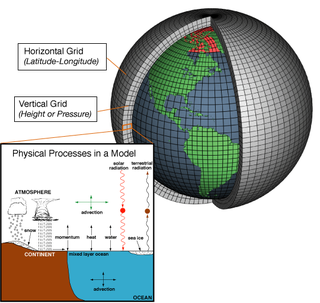
In atmospheric science, an atmospheric model is a mathematical model constructed around the full set of primitive, dynamical equations which govern atmospheric motions. It can supplement these equations with parameterizations for turbulent diffusion, radiation, moist processes, heat exchange, soil, vegetation, surface water, the kinematic effects of terrain, and convection. Most atmospheric models are numerical, i.e. they discretize equations of motion. They can predict microscale phenomena such as tornadoes and boundary layer eddies, sub-microscale turbulent flow over buildings, as well as synoptic and global flows. The horizontal domain of a model is either global, covering the entire Earth, or regional (limited-area), covering only part of the Earth. The different types of models run are thermotropic, barotropic, hydrostatic, and nonhydrostatic. Some of the model types make assumptions about the atmosphere which lengthens the time steps used and increases computational speed.

The central dense overcast, or CDO, of a tropical cyclone or strong subtropical cyclone is the large central area of thunderstorms surrounding its circulation center, caused by the formation of its eyewall. It can be round, angular, oval, or irregular in shape. This feature shows up in tropical cyclones of tropical storm or hurricane strength. How far the center is embedded within the CDO, and the temperature difference between the cloud tops within the CDO and the cyclone's eye, can help determine a tropical cyclone's intensity with the Dvorak technique. Locating the center within the CDO can be a problem with strong tropical storms and minimal hurricanes as its location can be obscured by the CDO's high cloud canopy. This center location problem can be resolved through the use of microwave satellite imagery.

Tropical cyclone forecasting is the science of forecasting where a tropical cyclone's center, and its effects, are expected to be at some point in the future. There are several elements to tropical cyclone forecasting: track forecasting, intensity forecasting, rainfall forecasting, storm surge, tornado, and seasonal forecasting. While skill is increasing in regard to track forecasting, intensity forecasting skill remains unchanged over the past several years. Seasonal forecasting began in the 1980s in the Atlantic basin and has spread into other basins in the years since.

Tropical cyclone track forecasting involves predicting where a tropical cyclone is going to track over the next five days, every 6 to 12 hours. The history of tropical cyclone track forecasting has evolved from a single-station approach to a comprehensive approach which uses a variety of meteorological tools and methods to make predictions. The weather of a particular location can show signs of the approaching tropical cyclone, such as increasing swell, increasing cloudiness, falling barometric pressure, increasing tides, squalls and heavy rainfall.

The quantitative precipitation forecast is the expected amount of melted precipitation accumulated over a specified time period over a specified area. A QPF will be created when precipitation amounts reaching a minimum threshold are expected during the forecast's valid period. Valid periods of precipitation forecasts are normally synoptic hours such as 00:00, 06:00, 12:00 and 18:00 GMT. Terrain is considered in QPFs by use of topography or based upon climatological precipitation patterns from observations with fine detail. Starting in the mid-to-late 1990s, QPFs were used within hydrologic forecast models to simulate impact to rivers throughout the United States. Forecast models show significant sensitivity to humidity levels within the planetary boundary layer, or in the lowest levels of the atmosphere, which decreases with height. QPF can be generated on a quantitative, forecasting amounts, or a qualitative, forecasting the probability of a specific amount, basis. Radar imagery forecasting techniques show higher skill than model forecasts within 6 to 7 hours of the time of the radar image. The forecasts can be verified through use of rain gauge measurements, weather radar estimates, or a combination of both. Various skill scores can be determined to measure the value of the rainfall forecast.
The maximum sustained wind associated with a tropical cyclone is a common indicator of the intensity of the storm. Within a mature tropical cyclone, it is found within the eyewall at a distance defined as the radius of maximum wind, or RMW. Unlike gusts, the value of these winds are determined via their sampling and averaging the sampled results over a period of time. Wind measuring has been standardized globally to reflect the winds at 10 metres (33 ft) above mean sea level, and the maximum sustained wind represents the highest average wind over either a one-minute (US) or ten-minute time span, anywhere within the tropical cyclone. Surface winds are highly variable due to friction between the atmosphere and the Earth's surface, as well as near hills and mountains over land.

Surface weather observations are the fundamental data used for safety as well as climatological reasons to forecast weather and issue warnings worldwide. They can be taken manually, by a weather observer, by computer through the use of automated weather stations, or in a hybrid scheme using weather observers to augment the otherwise automated weather station. The ICAO defines the International Standard Atmosphere (ISA), which is the model of the standard variation of pressure, temperature, density, and viscosity with altitude in the Earth's atmosphere, and is used to reduce a station pressure to sea level pressure. Airport observations can be transmitted worldwide through the use of the METAR observing code. Personal weather stations taking automated observations can transmit their data to the United States mesonet through the Citizen Weather Observer Program (CWOP), the UK Met Office through their Weather Observations Website (WOW), or internationally through the Weather Underground Internet site. A thirty-year average of a location's weather observations is traditionally used to determine the station's climate. In the US a network of Cooperative Observers make a daily record of summary weather and sometimes water level information.
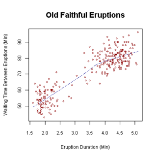
A plot is a graphical technique for representing a data set, usually as a graph showing the relationship between two or more variables. The plot can be drawn by hand or by a computer. In the past, sometimes mechanical or electronic plotters were used. Graphs are a visual representation of the relationship between variables, which are very useful for humans who can then quickly derive an understanding which may not have come from lists of values. Given a scale or ruler, graphs can also be used to read off the value of an unknown variable plotted as a function of a known one, but this can also be done with data presented in tabular form. Graphs of functions are used in mathematics, sciences, engineering, technology, finance, and other areas.
The following outline is provided as an overview of and topical guide to tropical cyclones:

The history of numerical weather prediction considers how current weather conditions as input into mathematical models of the atmosphere and oceans to predict the weather and future sea state has changed over the years. Though first attempted manually in the 1920s, it was not until the advent of the computer and computer simulation that computation time was reduced to less than the forecast period itself. ENIAC was used to create the first forecasts via computer in 1950, and over the years more powerful computers have been used to increase the size of initial datasets and use more complicated versions of the equations of motion. The development of global forecasting models led to the first climate models. The development of limited area (regional) models facilitated advances in forecasting the tracks of tropical cyclone as well as air quality in the 1970s and 1980s.
The following is a glossary of tropical cyclone terms.
Marine weather forecasting is the process by which mariners and meteorological organizations attempt to forecast future weather conditions over the Earth's oceans. Mariners have had rules of thumb regarding the navigation around tropical cyclones for many years, dividing a storm into halves and sailing through the normally weaker and more navigable half of their circulation. Marine weather forecasts by various weather organizations can be traced back to the sinking of the Royal Charter in 1859 and the RMS Titanic in 1912.
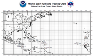
A tropical cyclone tracking chart is used by those within hurricane-threatened areas to track tropical cyclones worldwide. In the north Atlantic basin, they are known as hurricane tracking charts. New tropical cyclone information is available at least every six hours in the Northern Hemisphere and at least every twelve hours in the Southern Hemisphere. Charts include maps of the areas where tropical cyclones form and track within the various basins, include name lists for the year, basin-specific tropical cyclone definitions, rules of thumb for hurricane preparedness, emergency contact information, and numbers for figuring out where tropical cyclone shelters are open.

