In geodesy and geophysics, theoretical gravity or normal gravity is an approximation of the true gravity on Earth's surface by means of a mathematical model representing Earth. The most common model of a smoothed Earth is a rotating Earth ellipsoid of revolution (i.e., a spheroid).
Representations of gravity can be used in the study and analysis of other bodies, such as asteroids. Widely used representations of a gravity field in the context of geodesy include spherical harmonics, mascon models, and polyhedral gravity representations.[1]
The type of gravity model used for the Earth depends upon the degree of fidelity required for a given problem. For many problems such as aircraft simulation, it may be sufficient to consider gravity to be a constant, defined as:[2]
9.80665m/s2 (32.1740ft/s2)
based upon data from World Geodetic System 1984 (WGS-84), where is understood to be pointing 'down' in the local frame of reference.
If it is desirable to model an object's weight on Earth as a function of latitude, one could use the following:[2]:41
where
= 9.832m/s2 (32.26ft/s2)
= 9.806m/s2 (32.17ft/s2)
= 9.780m/s2 (32.09ft/s2)
= latitude, between −90° and +90°
Neither of these accounts for changes in gravity with changes in altitude, but the model with the cosine function does take into account the centrifugal relief that is produced by the rotation of the Earth. On the rotating sphere, the sum of the force of the gravitational field and the centrifugal force yields an angular deviation of approximately
(in radians) between the direction of the gravitational field and the direction measured by a plumb line; the plumb line appears to point southwards on the northern hemisphere and northwards on the southern hemisphere. rad/s is the diurnal angular speed of the Earth axis, and km the radius of the reference sphere, and the distance of the point on the Earth crust to the Earth axis. [3]
For the mass attraction effect by itself, the gravitational acceleration at the equator is about 0.18% less than that at the poles due to being located farther from the mass center. When the rotational component is included (as above), the gravity at the equator is about 0.53% less than that at the poles, with gravity at the poles being unaffected by the rotation. So the rotational component of change due to latitude (0.35%) is about twice as significant as the mass attraction change due to latitude (0.18%), but both reduce strength of gravity at the equator as compared to gravity at the poles.
Note that for satellites, orbits are decoupled from the rotation of the Earth so the orbital period is not necessarily one day, but also that errors can accumulate over multiple orbits so that accuracy is important. For such problems, the rotation of the Earth would be immaterial unless variations with longitude are modeled. Also, the variation in gravity with altitude becomes important, especially for highly elliptical orbits.
The Earth Gravitational Model 1996 (EGM96) contains 130,676 coefficients that refine the model of the Earth's gravitational field.[2]:40 The most significant correction term is about two orders of magnitude more significant than the next largest term.[2]:40 That coefficient is referred to as the term, and accounts for the flattening of the poles, or the oblateness, of the Earth. (A shape elongated on its axis of symmetry, like an American football, would be called prolate.) A gravitational potential function can be written for the change in potential energy for a unit mass that is brought from infinity into proximity to the Earth. Taking partial derivatives of that function with respect to a coordinate system will then resolve the directional components of the gravitational acceleration vector, as a function of location. The component due to the Earth's rotation can then be included, if appropriate, based on a sidereal day relative to the stars (≈366.24 days/year) rather than on a solar day (≈365.24 days/year). That component is perpendicular to the axis of rotation rather than to the surface of the Earth.
A similar model adjusted for the geometry and gravitational field for Mars can be found in publication NASA SP-8010.[4]
The barycentric gravitational acceleration at a point in space is given by:
where:
M is the mass of the attracting object, is the unit vector from center-of-mass of the attracting object to the center-of-mass of the object being accelerated, r is the distance between the two objects, and G is the gravitational constant.
When this calculation is done for objects on the surface of the Earth, or aircraft that rotate with the Earth, one has to account for the fact that the Earth is rotating and the centrifugal acceleration has to be subtracted from this. For example, the equation above gives the acceleration at 9.820m/s2, when GM = 3.986 × 10¹⁴ m3/s2, and R = 6.371 × 10⁶ m. The centripetal radius is r = R cos(φ), and the centripetal time unit is approximately (day / 2π), reduces this, for r = 5 × 10⁶ metres, to 9.79379m/s2, which is closer to the observed value. [citation needed]
Basic formulas
Various, successively more refined, formulas for computing the theoretical gravity are referred to as the International Gravity Formula, the first of which was proposed in 1930 by the International Association of Geodesy. The general shape of that formula is:
in which g(φ) is the gravity as a function of the geographic latitudeφ of the position whose gravity is to be determined, denotes the gravity at the equator (as determined by measurement), and the coefficients A and B are parameters that must be selected to produce a good global fit to true gravity.[5]
Using the values of the GRS80 reference system, a commonly used specific instantiation of the formula above is given by:
Up to the 1960s, formulas based on the Hayford ellipsoid (1924) and of the famous German geodesist Helmert (1906) were often used.[citation needed] The difference between the semi-major axis (equatorial radius) of the Hayford ellipsoid and that of the modern WGS84 ellipsoid is 251m; for Helmert's ellipsoid it is only 63m.
A more recent theoretical formula for gravity as a function of latitude is the International Gravity Formula 1980 (IGF80), also based on the GRS80 ellipsoid but now using the Somigliana equation (after Carlo Somigliana (1860–1955)[6]):
The normal gravity formula of Geodetic Reference System 1967 is defined with the values:
International gravity formula 1980
From the parameters of GRS 80 comes the classic series expansion:
The accuracy is about ±10−6 m/s2.
With GRS 80 the following series expansion is also introduced:
As such the parameters are:
c1= 5.2790414·10−3
c2= 2.32718·10−5
c3= 1.262·10−7
c4= 7·10−10
The accuracy is at about ±10−9 m/s2 exact. When the exactness is not required, the terms at further back can be omitted. But it is recommended to use this finalized formula.
Height dependence
Cassinis determined the height dependence, as:
The average rock densityρ is no longer considered.
The formula is based on the International gravity formula from1967.
The scale of free-fall acceleration at a certain place must be determined with precision measurement of several mechanical magnitudes. Weighing scales, the mass of which does measurement because of the weight, relies on the free-fall acceleration, thus for use they must be prepared with different constants in different places of use. Through the concept of so-called gravity zones, which are divided with the use of normal gravity, a weighing scale can be calibrated by the manufacturer before use.[9]
In mathematics and physics, Laplace's equation is a second-order partial differential equation named after Pierre-Simon Laplace, who first studied its properties. This is often written as
The Navier–Stokes equations are partial differential equations which describe the motion of viscous fluid substances. They were named after French engineer and physicist Claude-Louis Navier and the Irish physicist and mathematician George Gabriel Stokes. They were developed over several decades of progressively building the theories, from 1822 (Navier) to 1842–1850 (Stokes).
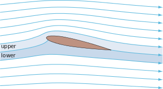
In fluid dynamics, potential flow or irrotational flow refers to a description of a fluid flow with no vorticity in it. Such a description typically arises in the limit of vanishing viscosity, i.e., for an inviscid fluid and with no vorticity present in the flow.
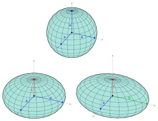
An ellipsoid is a surface that can be obtained from a sphere by deforming it by means of directional scalings, or more generally, of an affine transformation.
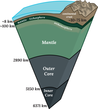
Earth radius is the distance from the center of Earth to a point on or near its surface. Approximating the figure of Earth by an Earth spheroid, the radius ranges from a maximum of nearly 6,378 km (3,963 mi) to a minimum of nearly 6,357 km (3,950 mi).
Geopotential is the potential of the Earth's gravity field. For convenience it is often defined as the negative of the potential energy per unit mass, so that the gravity vector is obtained as the gradient of the geopotential, without the negation. In addition to the actual potential, a hypothetical normal potential and their difference, the disturbing potential, can also be defined.
In mathematics, theta functions are special functions of several complex variables. They show up in many topics, including Abelian varieties, moduli spaces, quadratic forms, and solitons. As Grassmann algebras, they appear in quantum field theory.
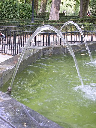
Projectile motion is a form of motion experienced by an object or particle that is projected in a gravitational field, such as from Earth's surface, and moves along a curved path under the action of gravity only. In the particular case of projectile motion on Earth, most calculations assume the effects of air resistance are passive and negligible. The curved path of objects in projectile motion was shown by Galileo to be a parabola, but may also be a straight line in the special case when it is thrown directly upward or downward. The study of such motions is called ballistics, and such a trajectory is a ballistic trajectory. The only force of mathematical significance that is actively exerted on the object is gravity, which acts downward, thus imparting to the object a downward acceleration towards the Earth’s center of mass. Because of the object's inertia, no external force is needed to maintain the horizontal velocity component of the object's motion. Taking other forces into account, such as aerodynamic drag or internal propulsion, requires additional analysis. A ballistic missile is a missile only guided during the relatively brief initial powered phase of flight, and whose remaining course is governed by the laws of classical mechanics.
In mathematics and physics, the Christoffel symbols are an array of numbers describing a metric connection. The metric connection is a specialization of the affine connection to surfaces or other manifolds endowed with a metric, allowing distances to be measured on that surface. In differential geometry, an affine connection can be defined without reference to a metric, and many additional concepts follow: parallel transport, covariant derivatives, geodesics, etc. also do not require the concept of a metric. However, when a metric is available, these concepts can be directly tied to the "shape" of the manifold itself; that shape is determined by how the tangent space is attached to the cotangent space by the metric tensor. Abstractly, one would say that the manifold has an associated (orthonormal) frame bundle, with each "frame" being a possible choice of a coordinate frame. An invariant metric implies that the structure group of the frame bundle is the orthogonal group O(p, q). As a result, such a manifold is necessarily a (pseudo-)Riemannian manifold. The Christoffel symbols provide a concrete representation of the connection of (pseudo-)Riemannian geometry in terms of coordinates on the manifold. Additional concepts, such as parallel transport, geodesics, etc. can then be expressed in terms of Christoffel symbols.
One of the guiding principles in modern chemical dynamics and spectroscopy is that the motion of the nuclei in a molecule is slow compared to that of its electrons. This is justified by the large disparity between the mass of an electron, and the typical mass of a nucleus and leads to the Born–Oppenheimer approximation and the idea that the structure and dynamics of a chemical species are largely determined by nuclear motion on potential energy surfaces.
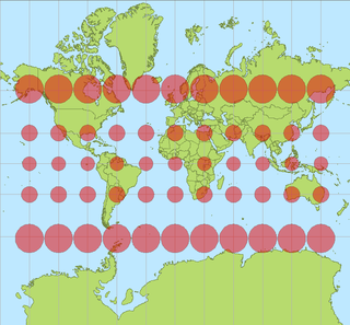
In cartography, a Tissot's indicatrix is a mathematical contrivance presented by French mathematician Nicolas Auguste Tissot in 1859 and 1871 in order to characterize local distortions due to map projection. It is the geometry that results from projecting a circle of infinitesimal radius from a curved geometric model, such as a globe, onto a map. Tissot proved that the resulting diagram is an ellipse whose axes indicate the two principal directions along which scale is maximal and minimal at that point on the map.
Great-circle navigation or orthodromic navigation is the practice of navigating a vessel along a great circle. Such routes yield the shortest distance between two points on the globe.
The gravity of Earth, denoted by g, is the net acceleration that is imparted to objects due to the combined effect of gravitation and the centrifugal force . It is a vector quantity, whose direction coincides with a plumb bob and strength or magnitude is given by the norm .
A pendulum is a body suspended from a fixed support so that it swings freely back and forth under the influence of gravity. When a pendulum is displaced sideways from its resting, equilibrium position, it is subject to a restoring force due to gravity that will accelerate it back towards the equilibrium position. When released, the restoring force acting on the pendulum's mass causes it to oscillate about the equilibrium position, swinging it back and forth. The mathematics of pendulums are in general quite complicated. Simplifying assumptions can be made, which in the case of a simple pendulum allow the equations of motion to be solved analytically for small-angle oscillations.
In general relativity, Lense–Thirring precession or the Lense–Thirring effect is a relativistic correction to the precession of a gyroscope near a large rotating mass such as the Earth. It is a gravitomagnetic frame-dragging effect. It is a prediction of general relativity consisting of secular precessions of the longitude of the ascending node and the argument of pericenter of a test particle freely orbiting a central spinning mass endowed with angular momentum .
In geodesy and navigation, a meridian arc is the curve between two points on the Earth's surface having the same longitude. The term may refer either to a segment of the meridian, or to its length.
In fluid dynamics, Luke's variational principle is a Lagrangian variational description of the motion of surface waves on a fluid with a free surface, under the action of gravity. This principle is named after J.C. Luke, who published it in 1967. This variational principle is for incompressible and inviscid potential flows, and is used to derive approximate wave models like the mild-slope equation, or using the averaged Lagrangian approach for wave propagation in inhomogeneous media.
In geophysics and physical geodesy, a geopotential model is the theoretical analysis of measuring and calculating the effects of Earth's gravitational field.
Lagrangian field theory is a formalism in classical field theory. It is the field-theoretic analogue of Lagrangian mechanics. Lagrangian mechanics is used to analyze the motion of a system of discrete particles each with a finite number of degrees of freedom. Lagrangian field theory applies to continua and fields, which have an infinite number of degrees of freedom.
Taylor–Maccoll flow refers to the steady flow behind a conical shock wave that is attached to a solid cone. The flow is named after G. I. Taylor and J. W. Maccoll, whom described the flow in 1933, guided by an earlier work of Theodore von Kármán.
↑ de Icaza-Herrera, M.; Castano, V. M. (2011). "Generalized Lagrangian of the parametric Foucault pendulum with dissipative forces". Acta Mech. 218: 45–64. doi:10.1007/s00707-010-0392-8.
↑ Richard B. Noll; Michael B. McElroy (1974), Models of Mars' Atmosphere [1974], Greenbelt, Maryland: NASA Goddard Space Flight Center, SP-8010.
This page is based on this Wikipedia article Text is available under the CC BY-SA 4.0 license; additional terms may apply. Images, videos and audio are available under their respective licenses.