Univariate (statistics)

Last updated

Univariate is a term commonly used in statistics to describe a type of data which consists of observations on only a single characteristic or attribute. A simple example of univariate data would be the salaries of workers in industry. [1] Like all the other data, univariate data can be visualized using graphs, images or other analysis tools after the data is measured, collected, reported, and analyzed. [2]

Contents

Univariate data types

Some univariate data consists of numbers (such as the height of 65 inches or the weight of 100 pounds), while others are nonnumerical (such as eye colors of brown or blue). Generally, the terms categorical univariate data and numerical univariate data are used to distinguish between these types.

Categorical univariate data

Categorical univariate data consists of non-numerical observations that may be placed in categories. It includes labels or names used to identify an attribute of each element. Categorical univariate data usually use either nominal or ordinal scale of measurement. [3]

Numerical univariate data

Numerical univariate data consists of observations that are numbers. They are obtained using either interval or ratio scale of measurement. This type of univariate data can be classified even further into two subcategories: discrete and continuous. [2] A numerical univariate data is discrete if the set of all possible values is finite or countably infinite. Discrete univariate data are usually associated with counting (such as the number of books read by a person). A numerical univariate data is continuous if the set of all possible values is an interval of numbers. Continuous univariate data are usually associated with measuring (such as the weights of people).

Data analysis and applications

Univariate analysis is the simplest form of analyzing data. Uni means "one", so the data has only one variable ( univariate ). [4] Univariate data requires to analyze each variable separately. Data is gathered for the purpose of answering a question, or more specifically, a research question. Univariate data does not answer research questions about relationships between variables, but rather it is used to describe one characteristic or attribute that varies from observation to observation. [5] Usually there are two purposes that a researcher can look for. The first one is to answer a research question with descriptive study and the second one is to get knowledge about how attribute varies with individual effect of a variable in regression analysis. There are some ways to describe patterns found in univariate data which include graphical methods, measures of central tendency and measures of variability. [6]

Like other forms of statistics, it can be inferential or descriptive. The key fact is that only one variable is involved.

Univariate analysis can yield misleading results in cases in which multivariate analysis is more appropriate.

Measures of central tendency

Central tendency is one of the most common numerical descriptive measures. It is used to estimate the central location of the univariate data by the calculation of mean, median and mode. [7] Each of these calculations has its own advantages and limitations. The mean has the advantage that its calculation includes each value of the data set, but it is particularly susceptible to the influence of outliers. The median is a better measure when the data set contains outliers. The mode is simple to locate.

One is not restricted to using only one of these measures of central tendency. If the data being analyzed is categorical, then the only measure of central tendency that can be used is the mode. However, if the data is numerical in nature (ordinal or interval/ratio) then the mode, median, or mean can all be used to describe the data. Using more than one of these measures provides a more accurate descriptive summary of central tendency for the univariate. [8]

Measures of variability

A measure of variability or dispersion (deviation from the mean) of a univariate data set can reveal the shape of a univariate data distribution more sufficiently. It will provide some information about the variation among data values. The measures of variability together with the measures of central tendency give a better picture of the data than the measures of central tendency alone. [9] The three most frequently used measures of variability are range, variance and standard deviation. [10] The appropriateness of each measure would depend on the type of data, the shape of the distribution of data and which measure of central tendency are being used. If the data is categorical, then there is no measure of variability to report. For data that is numerical, all three measures are possible. If the distribution of data is symmetrical, then the measures of variability are usually the variance and standard deviation. However, if the data are skewed, then the measure of variability that would be appropriate for that data set is the range. [3]

Descriptive methods

Descriptive statistics describe a sample or population. They can be part of exploratory data analysis. [11]

The appropriate statistic depends on the level of measurement. For nominal variables, a frequency table and a listing of the mode(s) is sufficient. For ordinal variables the median can be calculated as a measure of central tendency and the range (and variations of it) as a measure of dispersion. For interval level variables, the arithmetic mean (average) and standard deviation are added to the toolbox and, for ratio level variables, we add the geometric mean and harmonic mean as measures of central tendency and the coefficient of variation as a measure of dispersion.

For interval and ratio level data, further descriptors include the variable's skewness and kurtosis.

Inferential methods

Inferential methods allow us to infer from a sample to a population. [11] For a nominal variable a one-way chi-square (goodness of fit) test can help determine if our sample matches that of some population. [12] For interval and ratio level data, a one-sample t-test can let us infer whether the mean in our sample matches some proposed number (typically 0). Other available tests of location include the one-sample sign test and Wilcoxon signed rank test.

Graphical methods

The most frequently used graphical illustrations for univariate data are:

Frequency distribution tables

Frequency is how many times a number occurs. The frequency of an observation in statistics tells us the number of times the observation occurs in the data. For example, in the following list of numbers {1, 2, 3, 4, 6, 9, 9, 8, 5, 1, 1, 9, 9, 0, 6, 9}, the frequency of the number 9 is 5 (because it occurs 5 times in this data set).

Bar charts

This is an example of barplot. Barplot.jpg
This is an example of barplot.

Bar chart is a graph consisting of rectangular bars. These bars actually represents number or percentage of observations of existing categories in a variable. The length or height of bars gives a visual representation of the proportional differences among categories.

Histograms

histogram Histarman2.jpg
histogram

Histograms are used to estimate distribution of the data, with the frequency of values assigned to a value range called a bin. [13]

Pie charts

A pie chart Pie-chart.jpg
A pie chart

Pie chart is a circle divided into portions that represent the relative frequencies or percentages of a population or a sample belonging to different categories.

Univariate distributions

Univariate distribution is a dispersal type of a single random variable described either with a probability mass function (pmf) for discrete probability distribution, or probability density function (pdf) for continuous probability distribution. [14] It is not to be confused with multivariate distribution.

Common discrete distributions

Common continuous distributions

See also

Related Research Articles

In statistics, a central tendency is a central or typical value for a probability distribution.

<span class="mw-page-title-main">Descriptive statistics</span> Type of statistics

A descriptive statistic is a summary statistic that quantitatively describes or summarizes features from a collection of information, while descriptive statistics is the process of using and analysing those statistics. Descriptive statistics is distinguished from inferential statistics by its aim to summarize a sample, rather than use the data to learn about the population that the sample of data is thought to represent. This generally means that descriptive statistics, unlike inferential statistics, is not developed on the basis of probability theory, and are frequently nonparametric statistics. Even when a data analysis draws its main conclusions using inferential statistics, descriptive statistics are generally also presented. For example, in papers reporting on human subjects, typically a table is included giving the overall sample size, sample sizes in important subgroups, and demographic or clinical characteristics such as the average age, the proportion of subjects of each sex, the proportion of subjects with related co-morbidities, etc.

<span class="mw-page-title-main">Median</span> Middle quantile of a data set or probability distribution

The median of a set of numbers is the value separating the higher half from the lower half of a data sample, a population, or a probability distribution. For a data set, it may be thought of as the “middle" value. The basic feature of the median in describing data compared to the mean is that it is not skewed by a small proportion of extremely large or small values, and therefore provides a better representation of the center. Median income, for example, may be a better way to describe the center of the income distribution because increases in the largest incomes alone have no effect on the median. For this reason, the median is of central importance in robust statistics.

<span class="mw-page-title-main">Probability distribution</span> Mathematical function for the probability a given outcome occurs in an experiment

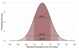
In probability theory and statistics, a probability distribution is the mathematical function that gives the probabilities of occurrence of different possible outcomes for an experiment. It is a mathematical description of a random phenomenon in terms of its sample space and the probabilities of events.

<span class="mw-page-title-main">Statistics</span> Study of the collection, analysis, interpretation, and presentation of data

Statistics is the discipline that concerns the collection, organization, analysis, interpretation, and presentation of data. In applying statistics to a scientific, industrial, or social problem, it is conventional to begin with a statistical population or a statistical model to be studied. Populations can be diverse groups of people or objects such as "all people living in a country" or "every atom composing a crystal". Statistics deals with every aspect of data, including the planning of data collection in terms of the design of surveys and experiments.

In statistics, a population is a set of similar items or events which is of interest for some question or experiment. A statistical population can be a group of existing objects or a hypothetical and potentially infinite group of objects conceived as a generalization from experience. A common aim of statistical analysis is to produce information about some chosen population.

The following outline is provided as an overview of and topical guide to statistics:

In statistics, a categorical variable is a variable that can take on one of a limited, and usually fixed, number of possible values, assigning each individual or other unit of observation to a particular group or nominal category on the basis of some qualitative property. In computer science and some branches of mathematics, categorical variables are referred to as enumerations or enumerated types. Commonly, each of the possible values of a categorical variable is referred to as a level. The probability distribution associated with a random categorical variable is called a categorical distribution.

<span class="mw-page-title-main">Mathematical statistics</span> Branch of statistics

Mathematical statistics is the application of probability theory, a branch of mathematics, to statistics, as opposed to techniques for collecting statistical data. Specific mathematical techniques which are used for this include mathematical analysis, linear algebra, stochastic analysis, differential equations, and measure theory.

In statistics, a contingency table is a type of table in a matrix format that displays the multivariate frequency distribution of the variables. They are heavily used in survey research, business intelligence, engineering, and scientific research. They provide a basic picture of the interrelation between two variables and can help find interactions between them. The term contingency table was first used by Karl Pearson in "On the Theory of Contingency and Its Relation to Association and Normal Correlation", part of the Drapers' Company Research Memoirs Biometric Series I published in 1904.

<span class="mw-page-title-main">Test statistic</span> Statistic used in statistical hypothesis testing

Test statistic is a quantity derived from the sample for statistical hypothesis testing. A hypothesis test is typically specified in terms of a test statistic, considered as a numerical summary of a data-set that reduces the data to one value that can be used to perform the hypothesis test. In general, a test statistic is selected or defined in such a way as to quantify, within observed data, behaviours that would distinguish the null from the alternative hypothesis, where such an alternative is prescribed, or that would characterize the null hypothesis if there is no explicitly stated alternative hypothesis.

In statistics, the mode is the value that appears most often in a set of data values. If X is a discrete random variable, the mode is the value x at which the probability mass function takes its maximum value. In other words, it is the value that is most likely to be sampled.

This glossary of statistics and probability is a list of definitions of terms and concepts used in the mathematical sciences of statistics and probability, their sub-disciplines, and related fields. For additional related terms, see Glossary of mathematics and Glossary of experimental design.

In statistics, the frequency or absolute frequency of an event is the number of times the observation has occurred/recorded in an experiment or study. These frequencies are often depicted graphically or in tabular form.

The mean absolute difference (univariate) is a measure of statistical dispersion equal to the average absolute difference of two independent values drawn from a probability distribution. A related statistic is the relative mean absolute difference, which is the mean absolute difference divided by the arithmetic mean, and equal to twice the Gini coefficient. The mean absolute difference is also known as the absolute mean difference and the Gini mean difference (GMD). The mean absolute difference is sometimes denoted by Δ or as MD.

In statistics, normality tests are used to determine if a data set is well-modeled by a normal distribution and to compute how likely it is for a random variable underlying the data set to be normally distributed.

<span class="mw-page-title-main">Statistical dispersion</span> Statistical property quantifying how much a collection of data is spread out

In statistics, dispersion is the extent to which a distribution is stretched or squeezed. Common examples of measures of statistical dispersion are the variance, standard deviation, and interquartile range. For instance, when the variance of data in a set is large, the data is widely scattered. On the other hand, when the variance is small, the data in the set is clustered.

<span class="mw-page-title-main">Bivariate analysis</span> Concept in statistical analysis

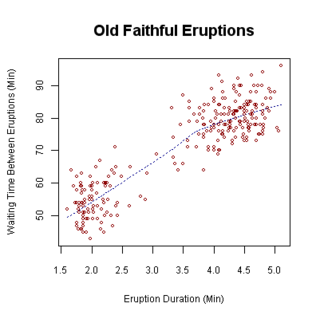
Bivariate analysis is one of the simplest forms of quantitative (statistical) analysis. It involves the analysis of two variables, for the purpose of determining the empirical relationship between them.

In statistics, groups of individual data points may be classified as belonging to any of various statistical data types, e.g. categorical ("red", "blue", "green"), real number (1.68, −5, 1.7×10+6), odd number (1,3,5) etc. The data type is a fundamental component of the semantic content of the variable, and controls which sorts of probability distributions can logically be used to describe the variable, the permissible operations on the variable, the type of regression analysis used to predict the variable, etc. The concept of data type is similar to the concept of level of measurement, but more specific: For example, count data require a different distribution (e.g. a Poisson distribution or binomial distribution) than non-negative real-valued data require, but both fall under the same level of measurement (a ratio scale).

References

  1. Kachigan, Sam Kash (1986). Statistical analysis : an interdisciplinary introduction to univariate & multivariate methods. New York: Radius Press. ISBN   0-942154-99-1.
  2. 1 2 Lacke, Prem S. Mann; with the help of Christopher Jay (2010). Introductory statistics (7th ed.). Hoboken, NJ: John Wiley & Sons. ISBN   978-0-470-44466-5.{{cite book}}: CS1 maint: multiple names: authors list (link)
  3. 1 2 Anderson, David R.; Sweeney, Dennis J.; Williams, Thomas A. Statistics For Business & Economics (Tenth ed.). Cengage Learning. p. 1018. ISBN   978-0-324-80926-8.
  4. "Univariate analysis". stathow.
  5. "Univariate Data". study.com.
  6. Trochim, William. "Descriptive Statistics". Web Center for Social Research Methods. Retrieved 15 February 2017.
  7. O'Rourke, Norm; Hatcher, Larry; Stepanski, Edward J. (2005). A step-by-step approach to using SAS for univariate & multivariate statistics (2nd ed.). New York: Wiley-Interscience. ISBN   1-59047-417-1.
  8. Longnecker, R. Lyman Ott, Michael (2009). An introduction to statistical methods and data analysis (6th ed., International ed.). Pacific Grove, Calif.: Brooks/Cole. ISBN   978-0-495-10914-3.{{cite book}}: CS1 maint: multiple names: authors list (link)
  9. Meloun, Milan; Militky, Jirí (2011). Statistical Data Analysis A Practical Guide. New Delhi: Woodhead Pub Ltd. ISBN   978-0-85709-109-3.
  10. Purves, David Freedman; Robert Pisani; Roger (2007). Statistics (4. ed.). New York [u.a.]: Norton. ISBN   978-0-393-92972-0.{{cite book}}: CS1 maint: multiple names: authors list (link)
  11. 1 2 Everitt, Brian (1998). The Cambridge Dictionary of Statistics . Cambridge, UK New York: Cambridge University Press. ISBN   0521593468.
  12. "One-Way Chi-Square".
  13. Diez, David M.; Barr, Christopher D.; Çetinkaya-Rundel, Mine (2015). OpenIntro Statistics (3rd ed.). OpenIntro, Inc. p. 30. ISBN   978-1-9434-5003-9.
  14. Samaniego, Francisco J. (2014). Stochastic modeling and mathematical statistics : a text for statisticians and quantitative scientists. Boca Raton: CRC Press. p. 167. ISBN   978-1-4665-6046-8.