Prefix sum

Last updated

In computer science, the prefix sum, cumulative sum, inclusive scan, or simply scan of a sequence of numbers x0, x1, x2, ... is a second sequence of numbers y0, y1, y2, ..., the sums of prefixes (running totals) of the input sequence:

Contents

y0 = x0
y1 = x0 + x1
y2 = x0 + x1+ x2
...

For instance, the prefix sums of the natural numbers are the triangular numbers:

input numbers 1 2 3 4 5 6...
prefix sums 1 3 6101521...

Prefix sums are trivial to compute in sequential models of computation, by using the formula yi = yi 1 + xi to compute each output value in sequence order. However, despite their ease of computation, prefix sums are a useful primitive in certain algorithms such as counting sort, [1] [2] and they form the basis of the scan higher-order function in functional programming languages. Prefix sums have also been much studied in parallel algorithms, both as a test problem to be solved and as a useful primitive to be used as a subroutine in other parallel algorithms. [3] [4] [5]

Abstractly, a prefix sum requires only a binary associative operator ⊕, making it useful for many applications from calculating well-separated pair decompositions of points to string processing. [6] [7]

Mathematically, the operation of taking prefix sums can be generalized from finite to infinite sequences; in that context, a prefix sum is known as a partial sum of a series. Prefix summation or partial summation form linear operators on the vector spaces of finite or infinite sequences; their inverses are finite difference operators.

Scan higher order function

In functional programming terms, the prefix sum may be generalized to any binary operation (not just the addition operation); the higher order function resulting from this generalization is called a scan, and it is closely related to the fold operation. Both the scan and the fold operations apply the given binary operation to the same sequence of values, but differ in that the scan returns the whole sequence of results from the binary operation, whereas the fold returns only the final result. For instance, the sequence of factorial numbers may be generated by a scan of the natural numbers using multiplication instead of addition:

input numbers123456...
prefix products12624120720...

Inclusive and exclusive scans

Programming language and library implementations of scan may be either inclusive or exclusive. An inclusive scan includes input xi when computing output yi (i.e., ) while an exclusive scan does not (i.e., ). In the latter case, implementations either leave y0 undefined or accept a separate "x−1" value with which to seed the scan. Either type of scan can be transformed into the other: an inclusive scan can be transformed into an exclusive scan by shifting the array produced by the scan right by one element and inserting the identity value at the left of the array. Conversely, an exclusive scan be transformed into an inclusive scan by shifting the array produced by the scan left and inserting the sum of the last element of the scan and the last element of the input array at the right of the array. [8]

The following table lists examples of the inclusive and exclusive scan functions provided by a few programming languages and libraries:

Language/libraryInclusive scanExclusive scan
APL +\
C++ std::inclusive_scanstd::exclusive_scan
Haskell scanl1 scanl
HPF sum_prefixsum_prefix(..., exclusive=.true.)
Kotlin scan
MPI MPI_ScanMPI_Exscan
Rust scan
Scala scan

The directive-based OpenMP parallel programming model supports both inclusive and exclusive scan support beginning with Version 5.0.

Parallel algorithms

There are two key algorithms for computing a prefix sum in parallel. The first offers a shorter span and more parallelism but is not work-efficient. The second is work-efficient but requires double the span and offers less parallelism. These are presented in turn below.

Algorithm 1: Shorter span, more parallel

Circuit representation of a highly parallel 16-input parallel prefix sum Hillis-Steele Prefix Sum.svg
Circuit representation of a highly parallel 16-input parallel prefix sum

Hillis and Steele present the following parallel prefix sum algorithm: [9]

fori <- 0 to floor(log2(n)) doforj <- 0 to n - 1 do in parallelifj < 2ithenxi+1
j
<- xi
j
elsexi+1
j
<- xi
j
+ xi
j - 2i

In the above, the notation means the value of the jth element of array x in timestep i.

With a single processor this algorithm would run in O(n log n) time. However if the machine has at least n processors to perform the inner loop in parallel, the algorithm as a whole runs in O(log n) time, the number of iterations of the outer loop.

Algorithm 2: Work-efficient

Circuit representation of a work-efficient 16-input parallel prefix sum Prefix sum 16.svg
Circuit representation of a work-efficient 16-input parallel prefix sum

A work-efficient parallel prefix sum can be computed by the following steps. [3] [10] [11]

  1. Compute the sums of consecutive pairs of items in which the first item of the pair has an even index: z0 = x0 + x1, z1 = x2 + x3, etc.
  2. Recursively compute the prefix sum w0, w1, w2, ... of the sequence z0, z1, z2, ...
  3. Express each term of the final sequence y0, y1, y2, ... as the sum of up to two terms of these intermediate sequences: y0 = x0, y1 = z0, y2 = z0 + x2, y3 = w1, etc. After the first value, each successive number yi is either copied from a position half as far through the w sequence, or is the previous value added to one value in the x sequence.

If the input sequence has n steps, then the recursion continues to a depth of O(log n), which is also the bound on the parallel running time of this algorithm. The number of steps of the algorithm is O(n), and it can be implemented on a parallel random access machine with O(n/log n) processors without any asymptotic slowdown by assigning multiple indices to each processor in rounds of the algorithm for which there are more elements than processors. [3]

Discussion

Each of the preceding algorithms runs in O(log n) time. However, the former takes exactly log2n steps, while the latter requires 2 log2 n 2 steps. For the 16-input examples illustrated, Algorithm 1 is 12-way parallel (49 units of work divided by a span of 4) while Algorithm 2 is only 4-way parallel (26 units of work divided by a span of 6). However, Algorithm 2 is work-efficientit performs only a constant factor (2) of the amount of work required by the sequential algorithmwhile Algorithm 1 is work-inefficientit performs asymptotically more work (a logarithmic factor) than is required sequentially. Consequently, Algorithm 1 is likely to perform better when abundant parallelism is available, but Algorithm 2 is likely to perform better when parallelism is more limited.

Parallel algorithms for prefix sums can often be generalized to other scan operations on associative binary operations, [3] [4] and they can also be computed efficiently on modern parallel hardware such as a GPU. [12] The idea of building in hardware a functional unit dedicated to computing multi-parameter prefix-sum was patented by Uzi Vishkin. [13]

Many parallel implementations follow a two pass procedure where partial prefix sums are calculated in the first pass on each processing unit; the prefix sum of these partial sums is then calculated and broadcast back to the processing units for a second pass using the now known prefix as the initial value. Asymptotically this method takes approximately two read operations and one write operation per item.

Concrete implementations of prefix sum algorithms

An implementation of a parallel prefix sum algorithm, like other parallel algorithms, has to take the parallelization architecture of the platform into account. More specifically, multiple algorithms exist which are adapted for platforms working on shared memory as well as algorithms which are well suited for platforms using distributed memory, relying on message passing as the only form of interprocess communication.

Shared memory: Two-level algorithm

The following algorithm assumes a shared memory machine model; all processing elements (PEs) have access to the same memory. A version of this algorithm is implemented in the Multi-Core Standard Template Library (MCSTL), [14] [15] a parallel implementation of the C++ standard template library which provides adapted versions for parallel computing of various algorithms.

In order to concurrently calculate the prefix sum over data elements with processing elements, the data is divided into blocks, each containing elements (for simplicity we assume that divides ). Note, that although the algorithm divides the data into blocks, only processing elements run in parallel at a time.

In a first sweep, each PE calculates a local prefix sum for its block. The last block does not need to be calculated, since these prefix sums are only calculated as offsets to the prefix sums of succeeding blocks and the last block is by definition not succeeded.

The offsets which are stored in the last position of each block are accumulated in a prefix sum of their own and stored in their succeeding positions. For being a small number, it is faster to do this sequentially, for a large , this step could be done in parallel as well.

A second sweep is performed. This time the first block does not have to be processed, since it does not need to account for the offset of a preceding block. However, in this sweep the last block is included instead and the prefix sums for each block are calculated taking the prefix sum block offsets calculated in the previous sweep into account.

functionprefix_sum(elements){n:=size(elements)p:=numberofprocessingelementsprefix_sum:=[0...0]ofsizendoparalleli=0top-1{// i := index of current PEfromj=i*n/(p+1)to(i+1)*n/(p+1)-1do{// This only stores the prefix sum of the local blocksstore_prefix_sum_with_offset_in(elements,0,prefix_sum)}}x=0fori=1top{// Serial accumulation of total sum of blocks x+=prefix_sum[i*n/(p+1)-1]// Build the prefix sum over the first p blocksprefix_sum[i*n/(p+1)]=x// Save the results to be used as offsets in second sweep}doparalleli=1top{// i := index of current PEfromj=i*n/(p+1)to(i+1)*n/(p+1)-1do{offset:=prefix_sum[i*n/(p+1)]// Calculate the prefix sum taking the sum of preceding blocks as offsetstore_prefix_sum_with_offset_in(elements,offset,prefix_sum)}}returnprefix_sum}

Improvement: In case that the number of blocks are too much that makes the serial step time-consuming by deploying a single processor, the Hillis and Steele algorithm can be used to accelerate the second phase.

Distributed memory: Hypercube algorithm

The Hypercube Prefix Sum Algorithm [16] is well adapted for distributed memory platforms and works with the exchange of messages between the processing elements. It assumes to have processor elements (PEs) participating in the algorithm equal to the number of corners in a -dimensional hypercube.

Different hypercubes for varying number of nodes Hypercube-construction-4d.png
Different hypercubes for varying number of nodes

Throughout the algorithm, each PE is seen as a corner in a hypothetical hyper cube with knowledge of the total prefix sum as well as the prefix sum of all elements up to itself (according to the ordered indices among the PEs), both in its own hypercube.

  • The algorithm starts by assuming every PE is the single corner of a zero dimensional hyper cube and therefore and are equal to the local prefix sum of its own elements.
  • The algorithm goes on by unifying hypercubes which are adjacent along one dimension. During each unification, is exchanged and aggregated between the two hyper cubes which keeps the invariant that all PEs at corners of this new hyper cube store the total prefix sum of this newly unified hyper cube in their variable . However, only the hyper cube containing the PEs with higher index also adds this to their local variable , keeping the invariant that only stores the value of the prefix sum of all elements at PEs with indices smaller or equal to their own index.

In a -dimensional hyper cube with PEs at the corners, the algorithm has to be repeated times to have the zero-dimensional hyper cubes be unified into one -dimensional hyper cube. Assuming a duplex communication model where the of two adjacent PEs in different hyper cubes can be exchanged in both directions in one communication step, this means communication startups.

i:=Indexofownprocessorelement(PE)m:=prefixsumoflocalelementsofthisPEd:=numberofdimensionsofthehypercubex=m;// Invariant: The prefix sum up to this PE in the current sub cubeσ=m;// Invariant: The prefix sum of all elements in the current sub cubefor(k=0;k<=d-1;k++){y=σ@PE(ixor2^k)// Get the total prefix sum of the opposing sub cube along dimension kσ=σ+y// Aggregate the prefix sum of both sub cubesif(i&2^k){x=x+y// Only aggregate the prefix sum from the other sub cube, if this PE is the higher index one.}}

Large message sizes: pipelined binary tree

The Pipelined Binary Tree Algorithm [17] is another algorithm for distributed memory platforms which is specifically well suited for large message sizes.

Like the hypercube algorithm, it assumes a special communication structure. The processing elements (PEs) are hypothetically arranged in a binary tree (e.g. a Fibonacci Tree) with infix numeration according to their index within the PEs. Communication on such a tree always occurs between parent and child nodes.

The infix numeration ensures that for any given PEj, the indices of all nodes reachable by its left subtree are less than and the indices of all nodes in the right subtree are greater than . The parent's index is greater than any of the indices in PEj's subtree if PEj is a left child and smaller if PEj is a right child. This allows for the following reasoning:

Information exchange between processing elements during upward (blue) and downward (red) phase in the Pipelined Binary Tree Prefix Sum algorithm. Pipelined Binary Tree Prefix Sum Communication.png
Information exchange between processing elements during upward (blue) and downward (red) phase in the Pipelined Binary Tree Prefix Sum algorithm.
  • The local prefix sum of the left subtree has to be aggregated to calculate PEj's local prefix sum .
  • The local prefix sum of the right subtree has to be aggregated to calculate the local prefix sum of higher level PEh which are reached on a path containing a left children connection (which means ).
  • The total prefix sum of PEj is necessary to calculate the total prefix sums in the right subtree (e.g. for the highest index node in the subtree).
  • PEj needs to include the total prefix sum of the first higher order node which is reached via an upward path including a right children connection to calculate its total prefix sum.

Note the distinction between subtree-local and total prefix sums. The points two, three and four can lead to believe they would form a circular dependency, but this is not the case. Lower level PEs might require the total prefix sum of higher level PEs to calculate their total prefix sum, but higher level PEs only require subtree local prefix sums to calculate their total prefix sum. The root node as highest level node only requires the local prefix sum of its left subtree to calculate its own prefix sum. Each PE on the path from PE0 to the root PE only requires the local prefix sum of its left subtree to calculate its own prefix sum, whereas every node on the path from PEp-1 (last PE) to the PEroot requires the total prefix sum of its parent to calculate its own total prefix sum.

This leads to a two-phase algorithm:

Upward Phase
Propagate the subtree local prefix sum to its parent for each PEj.

Downward phase
Propagate the exclusive (exclusive PEj as well as the PEs in its left subtree) total prefix sum of all lower index PEs which are not included in the addressed subtree of PEj to lower level PEs in the left child subtree of PEj. Propagate the inclusive prefix sum to the right child subtree of PEj.

Note that the algorithm is run in parallel at each PE and the PEs will block upon receive until their children/parents provide them with packets.

k:=numberofpacketsinamessagemofaPEm@{left,right,parent,this}:=// Messages at the different PEsx=m@this// Upward phase - Calculate subtree local prefix sumsforj=0tok-1:// Pipelining: For each packet of a messageifhasLeftChild:blockingreceivem[j]@left// This replaces the local m[j] with the received m[j]// Aggregate inclusive local prefix sum from lower index PEsx[j]=m[j]x[j]ifhasRightChild:blockingreceivem[j]@right// We do not aggregate m[j] into the local prefix sum, since the right children are higher index PEssendx[j]m[j]toparentelse:sendx[j]toparent// Downward phaseforj=0tok-1:m[j]@this=0ifhasParent:blockingreceivem[j]@parent// For a left child m[j] is the parents exclusive prefix sum, for a right child the inclusive prefix sumx[j]=m[j]x[j]sendm[j]toleft// The total prefix sum of all PE's smaller than this or any PE in the left subtreesendx[j]toright// The total prefix sum of all PE's smaller or equal than this PE
Pipelining

If the message m of length n can be divided into k packets and the operator ⨁ can be used on each of the corresponding message packets separately, pipelining is possible. [17]

If the algorithm is used without pipelining, there are always only two levels (the sending PEs and the receiving PEs) of the binary tree at work while all other PEs are waiting. If there are p processing elements and a balanced binary tree is used, the tree has levels, the length of the path from to is therefore which represents the maximum number of non parallel communication operations during the upward phase, likewise, the communication on the downward path is also limited to startups. Assuming a communication startup time of and a bytewise transmission time of , upward and downward phase are limited to in a non pipelined scenario.

Upon division into k packets, each of size and sending them separately, the first packet still needs to be propagated to as part of a local prefix sum and this will occur again for the last packet if . However, in between, all the PEs along the path can work in parallel and each third communication operation (receive left, receive right, send to parent) sends a packet to the next level, so that one phase can be completed in communication operations and both phases together need which is favourable for large message sizes n.

The algorithm can further be optimised by making use of full-duplex or telephone model communication and overlapping the upward and the downward phase. [17]

Data structures

When a data set may be updated dynamically, it may be stored in a Fenwick tree data structure. This structure allows both the lookup of any individual prefix sum value and the modification of any array value in logarithmic time per operation. [18] However, an earlier 1982 paper [19] presents a data structure called Partial Sums Tree (see Section 5.1) that appears to overlap Fenwick trees; in 1982 the term prefix-sum was not yet as common as it is today.

For higher-dimensional arrays, the summed area table provides a data structure based on prefix sums for computing sums of arbitrary rectangular subarrays. This can be a helpful primitive in image convolution operations. [20]

Applications

Counting sort is an integer sorting algorithm that uses the prefix sum of a histogram of key frequencies to calculate the position of each key in the sorted output array. It runs in linear time for integer keys that are smaller than the number of items, and is frequently used as part of radix sort, a fast algorithm for sorting integers that are less restricted in magnitude. [1]

List ranking, the problem of transforming a linked list into an array that represents the same sequence of items, can be viewed as computing a prefix sum on the sequence 1, 1, 1, ... and then mapping each item to the array position given by its prefix sum value; by combining list ranking, prefix sums, and Euler tours, many important problems on trees may be solved by efficient parallel algorithms. [4]

An early application of parallel prefix sum algorithms was in the design of binary adders, Boolean circuits that can add two n-bit binary numbers. In this application, the sequence of carry bits of the addition can be represented as a scan operation on the sequence of pairs of input bits, using the majority function to combine the previous carry with these two bits. Each bit of the output number can then be found as the exclusive or of two input bits with the corresponding carry bit. By using a circuit that performs the operations of the parallel prefix sum algorithm, it is possible to design an adder that uses O(n) logic gates and O(log n) time steps. [3] [10] [11]

In the parallel random access machine model of computing, prefix sums can be used to simulate parallel algorithms that assume the ability for multiple processors to access the same memory cell at the same time, on parallel machines that forbid simultaneous access. By means of a sorting network, a set of parallel memory access requests can be ordered into a sequence such that accesses to the same cell are contiguous within the sequence; scan operations can then be used to determine which of the accesses succeed in writing to their requested cells, and to distribute the results of memory read operations to multiple processors that request the same result. [21]

In Guy Blelloch's Ph.D. thesis, [22] parallel prefix operations form part of the formalization of the data parallelism model provided by machines such as the Connection Machine. The Connection Machine CM-1 and CM-2 provided a hypercubic network on which the Algorithm 1 above could be implemented, whereas the CM-5 provided a dedicated network to implement Algorithm 2. [23]

In the construction of Gray codes, sequences of binary values with the property that consecutive sequence values differ from each other in a single bit position, a number n can be converted into the Gray code value at position n of the sequence simply by taking the exclusive or of n and n/2 (the number formed by shifting n right by a single bit position). The reverse operation, decoding a Gray-coded value x into a binary number, is more complicated, but can be expressed as the prefix sum of the bits of x, where each summation operation within the prefix sum is performed modulo two. A prefix sum of this type may be performed efficiently using the bitwise Boolean operations available on modern computers, by computing the exclusive or of x with each of the numbers formed by shifting x to the left by a number of bits that is a power of two. [24]

Parallel prefix (using multiplication as the underlying associative operation) can also be used to build fast algorithms for parallel polynomial interpolation. In particular, it can be used to compute the divided difference coefficients of the Newton form of the interpolation polynomial. [25] This prefix based approach can also be used to obtain the generalized divided differences for (confluent) Hermite interpolation as well as for parallel algorithms for Vandermonde systems. [26]

Prefix sum is used for load balancing as a low-cost algorithm to distribute the work between multiple processors, where the overriding goal is achieving an equal amount of work on each processor. The algorithms uses an array of weights representing the amount of work required for each item. After the prefix sum is calculated, the work item i is sent for processing to the processor unit with the number . [27] Graphically this corresponds to an operation where the amount of work in each item is represented by the length of a linear segment, all segments are sequentially placed onto a line and the result cut into number of pieces, corresponding to the number of the processors. [28]

See also

Related Research Articles

<span class="mw-page-title-main">Merge sort</span> Divide and conquer sorting algorithm

In computer science, merge sort is an efficient, general-purpose, and comparison-based sorting algorithm. Most implementations produce a stable sort, which means that the relative order of equal elements is the same in the input and output. Merge sort is a divide-and-conquer algorithm that was invented by John von Neumann in 1945. A detailed description and analysis of bottom-up merge sort appeared in a report by Goldstine and von Neumann as early as 1948.

A splay tree is a binary search tree with the additional property that recently accessed elements are quick to access again. Like self-balancing binary search trees, a splay tree performs basic operations such as insertion, look-up and removal in O(log n) amortized time. For random access patterns drawn from a non-uniform random distribution, their amortized time can be faster than logarithmic, proportional to the entropy of the access pattern. For many patterns of non-random operations, also, splay trees can take better than logarithmic time, without requiring advance knowledge of the pattern. According to the unproven dynamic optimality conjecture, their performance on all access patterns is within a constant factor of the best possible performance that could be achieved by any other self-adjusting binary search tree, even one selected to fit that pattern. The splay tree was invented by Daniel Sleator and Robert Tarjan in 1985.

<span class="mw-page-title-main">Treap</span>

In computer science, the treap and the randomized binary search tree are two closely related forms of binary search tree data structures that maintain a dynamic set of ordered keys and allow binary searches among the keys. After any sequence of insertions and deletions of keys, the shape of the tree is a random variable with the same probability distribution as a random binary tree; in particular, with high probability its height is proportional to the logarithm of the number of keys, so that each search, insertion, or deletion operation takes logarithmic time to perform.

In computer science, a topological sort or topological ordering of a directed graph is a linear ordering of its vertices such that for every directed edge (u,v) from vertex u to vertex v, u comes before v in the ordering. For instance, the vertices of the graph may represent tasks to be performed, and the edges may represent constraints that one task must be performed before another; in this application, a topological ordering is just a valid sequence for the tasks. Precisely, a topological sort is a graph traversal in which each node v is visited only after all its dependencies are visited. A topological ordering is possible if and only if the graph has no directed cycles, that is, if it is a directed acyclic graph (DAG). Any DAG has at least one topological ordering, and algorithms are known for constructing a topological ordering of any DAG in linear time. Topological sorting has many applications, especially in ranking problems such as feedback arc set. Topological sorting is possible even when the DAG has disconnected components.

In computer science, a disjoint-set data structure, also called a union–find data structure or merge–find set, is a data structure that stores a collection of disjoint (non-overlapping) sets. Equivalently, it stores a partition of a set into disjoint subsets. It provides operations for adding new sets, merging sets, and finding a representative member of a set. The last operation makes it possible to find out efficiently if any two elements are in the same or different sets.

In computer science, a fusion tree is a type of tree data structure that implements an associative array on w-bit integers on a finite universe, where each of the input integers has size less than 2w and is non-negative. When operating on a collection of n key–value pairs, it uses O(n) space and performs searches in O(logwn) time, which is asymptotically faster than a traditional self-balancing binary search tree, and also better than the van Emde Boas tree for large values of w. It achieves this speed by using certain constant-time operations that can be done on a machine word. Fusion trees were invented in 1990 by Michael Fredman and Dan Willard.

<i>m</i>-ary tree Tree data structure in which each node has at most m children.

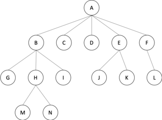
In graph theory, an m-ary tree is an arborescence in which each node has no more than m children. A binary tree is the special case where m = 2, and a ternary tree is another case with m = 3 that limits its children to three.

Intuitively, an algorithmically random sequence is a sequence of binary digits that appears random to any algorithm running on a universal Turing machine. The notion can be applied analogously to sequences on any finite alphabet. Random sequences are key objects of study in algorithmic information theory.

<span class="mw-page-title-main">Data parallelism</span> Parallelization across multiple processors in parallel computing environments

Data parallelism is parallelization across multiple processors in parallel computing environments. It focuses on distributing the data across different nodes, which operate on the data in parallel. It can be applied on regular data structures like arrays and matrices by working on each element in parallel. It contrasts to task parallelism as another form of parallelism.

The block Wiedemann algorithm for computing kernel vectors of a matrix over a finite field is a generalization by Don Coppersmith of an algorithm due to Doug Wiedemann.

Samplesort is a sorting algorithm that is a divide and conquer algorithm often used in parallel processing systems. Conventional divide and conquer sorting algorithms partitions the array into sub-intervals or buckets. The buckets are then sorted individually and then concatenated together. However, if the array is non-uniformly distributed, the performance of these sorting algorithms can be significantly throttled. Samplesort addresses this issue by selecting a sample of size s from the n-element sequence, and determining the range of the buckets by sorting the sample and choosing p−1 < s elements from the result. These elements then divide the array into p approximately equal-sized buckets. Samplesort is described in the 1970 paper, "Samplesort: A Sampling Approach to Minimal Storage Tree Sorting", by W. D. Frazer and A. C. McKellar.

<span class="mw-page-title-main">Fenwick tree</span> Data structure

A Fenwick tree or binary indexed tree(BIT) is a data structure that can efficiently update values and calculate prefix sums in an array of values.

Collective operations are building blocks for interaction patterns, that are often used in SPMD algorithms in the parallel programming context. Hence, there is an interest in efficient realizations of these operations.

In computer science, an optimal binary search tree (Optimal BST), sometimes called a weight-balanced binary tree, is a binary search tree which provides the smallest possible search time (or expected search time) for a given sequence of accesses (or access probabilities). Optimal BSTs are generally divided into two types: static and dynamic.

In computer science, parallel tree contraction is a broadly applicable technique for the parallel solution of a large number of tree problems, and is used as an algorithm design technique for the design of a large number of parallel graph algorithms. Parallel tree contraction was introduced by Gary L. Miller and John H. Reif, and has subsequently been modified to improve efficiency by X. He and Y. Yesha, Hillel Gazit, Gary L. Miller and Shang-Hua Teng and many others.

In computer science, the reduction operator is a type of operator that is commonly used in parallel programming to reduce the elements of an array into a single result. Reduction operators are associative and often commutative. The reduction of sets of elements is an integral part of programming models such as Map Reduce, where a reduction operator is applied (mapped) to all elements before they are reduced. Other parallel algorithms use reduction operators as primary operations to solve more complex problems. Many reduction operators can be used for broadcasting to distribute data to all processors.

The two-tree broadcast is an algorithm that implements a broadcast communication pattern on a distributed system using message passing. A broadcast is a commonly used collective operation that sends data from one processor to all other processors. The two-tree broadcast communicates concurrently over two binary trees that span all processors. This achieves full usage of the bandwidth in the full-duplex communication model while having a startup latency logarithmic in the number of partaking processors. The algorithm can also be adapted to perform a reduction or prefix sum.

A central problem in algorithmic graph theory is the shortest path problem. Hereby, the problem of finding the shortest path between every pair of nodes is known as all-pair-shortest-paths (APSP) problem. As sequential algorithms for this problem often yield long runtimes, parallelization has shown to be beneficial in this field. In this article two efficient algorithms solving this problem are introduced.

<span class="mw-page-title-main">Parallel external memory</span>

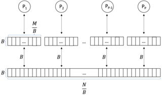
In computer science, a parallel external memory (PEM) model is a cache-aware, external-memory abstract machine. It is the parallel-computing analogy to the single-processor external memory (EM) model. In a similar way, it is the cache-aware analogy to the parallel random-access machine (PRAM). The PEM model consists of a number of processors, together with their respective private caches and a shared main memory.

-dimensional hypercube is a network topology for parallel computers with processing elements. The topology allows for an efficient implementation of some basic communication primitives such as Broadcast, All-Reduce, and Prefix sum. The processing elements are numbered through . Each processing element is adjacent to processing elements whose numbers differ in one and only one bit. The algorithms described in this page utilize this structure efficiently.

References

  1. 1 2 Cormen, Thomas H.; Leiserson, Charles E.; Rivest, Ronald L.; Stein, Clifford (2001), "8.2 Counting Sort", Introduction to Algorithms (2nd ed.), MIT Press and McGraw-Hill, pp. 168–170, ISBN   0-262-03293-7 .
  2. Cole, Richard; Vishkin, Uzi (1986), "Deterministic coin tossing with applications to optimal parallel list ranking", Information and Control, 70 (1): 32–53, doi: 10.1016/S0019-9958(86)80023-7
  3. 1 2 3 4 5 Ladner, R. E.; Fischer, M. J. (1980), "Parallel Prefix Computation", Journal of the ACM , 27 (4): 831–838, CiteSeerX   10.1.1.106.6247 , doi:10.1145/322217.322232, MR   0594702, S2CID   207568668 .
  4. 1 2 3 Tarjan, Robert E.; Vishkin, Uzi (1985), "An efficient parallel biconnectivity algorithm", SIAM Journal on Computing , 14 (4): 862–874, CiteSeerX   10.1.1.465.8898 , doi:10.1137/0214061 .
  5. Lakshmivarahan, S.; Dhall, S.K. (1994), Parallelism in the Prefix Problem , Oxford University Press, ISBN   0-19508849-2 .
  6. Blelloch, Guy (2011), Prefix Sums and Their Applications (Lecture Notes) (PDF), Carnegie Mellon University.
  7. Callahan, Paul; Kosaraju, S. Rao (1995), "A Decomposition of Multi-Dimensional Point Sets with Applications to k-Nearest-Neighbors and n-Body Potential Fields", Journal of the ACM, 42 (1): 67–90, doi: 10.1145/200836.200853 , S2CID   1818562 .
  8. "GPU Gems 3".
  9. Hillis, W. Daniel; Steele, Jr., Guy L. (December 1986). "Data parallel algorithms". Communications of the ACM. 29 (12): 1170–1183. doi: 10.1145/7902.7903 .
  10. 1 2 Ofman, Yu. (1962), Об алгоритмической сложности дискретных функций, Doklady Akademii Nauk SSSR (in Russian), 145 (1): 48–51, MR   0168423 . English translation, "On the algorithmic complexity of discrete functions", Soviet Physics Doklady7: 589–591 1963.
  11. 1 2 Khrapchenko, V. M. (1967), "Asymptotic Estimation of Addition Time of a Parallel Adder", Problemy Kibernet. (in Russian), 19: 107–122. English translation in Syst. Theory Res.19; 105–122, 1970.
  12. Sengupta, Shubhabrata; Harris, Mark; Zhang, Yao; Owens, John D. (2007). Scan primitives for GPU computing. Proc. 22nd ACM SIGGRAPH/EUROGRAPHICS Symposium on Graphics Hardware. pp. 97–106. Archived from the original on 2014-09-03. Retrieved 2007-11-29.
  13. Vishkin, Uzi (2003). Prefix sums and an application thereof. U.S. Patent 6,542,918.
  14. Singler, Johannes. "MCSTL: The Multi-Core Standard Template Library" . Retrieved 2019-03-29.
  15. Singler, Johannes; Sanders, Peter; Putze, Felix (2007). "MCSTL: The Multi-core Standard Template Library". Euro-Par 2007 Parallel Processing. Lecture Notes in Computer Science. Vol. 4641. pp. 682–694. doi:10.1007/978-3-540-74466-5_72. ISBN   978-3-540-74465-8. ISSN   0302-9743.
  16. Ananth Grama; Vipin Kumar; Anshul Gupta (2003). Introduction to Parallel Computing. Addison-Wesley. pp. 85, 86. ISBN   978-0-201-64865-2.
  17. 1 2 3 Sanders, Peter; Träff, Jesper Larsson (2006). "Parallel Prefix (Scan) Algorithms for MPI". Recent Advances in Parallel Virtual Machine and Message Passing Interface. Lecture Notes in Computer Science. Vol. 4192. pp. 49–57. doi:10.1007/11846802_15. ISBN   978-3-540-39110-4. ISSN   0302-9743.
  18. Fenwick, Peter M. (1994), "A new data structure for cumulative frequency tables", Software: Practice and Experience, 24 (3): 327–336, doi:10.1002/spe.4380240306, S2CID   7519761
  19. Shiloach, Yossi; Vishkin, Uzi (1982b), "An O(n2 log n) parallel max-flow algorithm", Journal of Algorithms, 3 (2): 128–146, doi:10.1016/0196-6774(82)90013-X
  20. Szeliski, Richard (2010), "Summed area table (integral image)", Computer Vision: Algorithms and Applications, Texts in Computer Science, Springer, pp. 106–107, ISBN   9781848829350 .
  21. Vishkin, Uzi (1983), "Implementation of simultaneous memory address access in models that forbid it", Journal of Algorithms, 4 (1): 45–50, doi:10.1016/0196-6774(83)90033-0, MR   0689265 .
  22. Blelloch, Guy E. (1990). Vector models for data-parallel computing . Cambridge, MA: MIT Press. ISBN   026202313X. OCLC   21761743.
  23. Leiserson, Charles E.; Abuhamdeh, Zahi S.; Douglas, David C.; Feynman, Carl R.; Ganmukhi, Mahesh N.; Hill, Jeffrey V.; Hillis, W. Daniel; Kuszmaul, Bradley C.; St. Pierre, Margaret A. (March 15, 1996). "The Network Architecture of the Connection Machine CM-5". Journal of Parallel and Distributed Computing. 33 (2): 145–158. doi:10.1006/jpdc.1996.0033. ISSN   0743-7315.
  24. Warren, Henry S. (2003), Hacker's Delight, Addison-Wesley, p. 236, ISBN   978-0-201-91465-8 .
  25. Eğecioğlu, O.; Gallopoulos, E.; Koç, C. (1990), "A parallel method for fast and practical high-order Newton interpolation", BIT Computer Science and Numerical Mathematics, 30 (2): 268–288, doi:10.1007/BF02017348, S2CID   9607531 .
  26. Eğecioğlu, O.; Gallopoulos, E.; Koç, C. (1989), "Fast computation of divided differences and parallel Hermite interpolation", Journal of Complexity, 5 (4): 417–437, doi:10.1016/0885-064X(89)90018-6
  27. Becker, Aaron; Zheng, Gengbin; Kalé, Laxmikant V. (2011). "Load Balancing, Distributed Memory". Encyclopedia of Parallel Computing. Boston, MA: Springer US. p. 1046. doi:10.1007/978-0-387-09766-4_504. ISBN   978-0-387-09765-7.
  28. Sanders, Peter; Mehlhorn, Kurt; Dietzfelbinger, Martin; Dementiev, Roman (2019). "Load Balancing" (PDF). Sequential and Parallel Algorithms and Data Structures. Cham: Springer International Publishing. p. 419–434. doi:10.1007/978-3-030-25209-0_14. ISBN   978-3-030-25208-3.