Binary tree

Last updated
A labeled binary tree of size 9 (the number of nodes in the tree) and height 3 (the height of a tree defined as the number of edges or links from the top-most or root node to the farthest leaf node), with a root node whose value is 1. The above tree is unbalanced and not sorted. Binary tree v2.svg
A labeled binary tree of size 9 (the number of nodes in the tree) and height 3 (the height of a tree defined as the number of edges or links from the top-most or root node to the farthest leaf node), with a root node whose value is 1. The above tree is unbalanced and not sorted.

In computer science, a binary tree is a tree data structure in which each node has at most two children, referred to as the left child and the right child. That is, it is a k-ary tree with k = 2. A recursive definition using set theory is that a binary tree is a tuple (L, S, R), where L and R are binary trees or the empty set and S is a singleton set containing the root. [1] [2]

Contents

From a graph theory perspective, binary trees as defined here are arborescences. [3] A binary tree may thus be also called a bifurcating arborescence, [3] a term which appears in some early programming books [4] before the modern computer science terminology prevailed. It is also possible to interpret a binary tree as an undirected, rather than directed graph, in which case a binary tree is an ordered, rooted tree. [5] Some authors use rooted binary tree instead of binary tree to emphasize the fact that the tree is rooted, but as defined above, a binary tree is always rooted. [6]

In mathematics, what is termed binary tree can vary significantly from author to author. Some use the definition commonly used in computer science, [7] but others define it as every non-leaf having exactly two children and don't necessarily label the children as left and right either. [8]

In computing, binary trees can be used in two very different ways:

Definitions

Recursive definition

To define a binary tree, the possibility that only one of the children may be empty must be acknowledged. An artifact, which in some textbooks is called an extended binary tree, is needed for that purpose. An extended binary tree is thus recursively defined as: [11]

Another way of imagining this construction (and understanding the terminology) is to consider instead of the empty set a different type of node—for instance square nodes if the regular ones are circles. [12]

Using graph theory concepts

A binary tree is a rooted tree that is also an ordered tree (a.k.a. plane tree) in which every node has at most two children. A rooted tree naturally imparts a notion of levels (distance from the root); thus, for every node, a notion of children may be defined as the nodes connected to it a level below. Ordering of these children (e.g., by drawing them on a plane) makes it possible to distinguish a left child from a right child. [13] But this still does not distinguish between a node with left but not a right child from a node with right but no left child.

The necessary distinction can be made by first partitioning the edges; i.e., defining the binary tree as triplet (V, E1, E2), where (V, E1 ∪ E2) is a rooted tree (equivalently arborescence) and E1 ∩ E2 is empty, and also requiring that for all j ∈ { 1, 2 }, every node has at most one Ej child. [14] A more informal way of making the distinction is to say, quoting the Encyclopedia of Mathematics, that "every node has a left child, a right child, neither, or both" and to specify that these "are all different" binary trees. [7]

Types of binary trees

Tree terminology is not well-standardized and so varies in literatures.

A full binary tree Full binary.svg
A full binary tree
An ancestry chart which can be mapped to a perfect 4-level binary tree. Waldburg Ahnentafel.jpg
An ancestry chart which can be mapped to a perfect 4-level binary tree.
A complete binary tree (that is not full) Complete binary2.svg
A complete binary tree (that is not full)

Properties of binary trees

Combinatorics

In combinatorics, one considers the problem of counting the number of full binary trees of a given size. Here the trees have no values attached to their nodes (this would just multiply the number of possible trees by an easily determined factor), and trees are distinguished only by their structure; however, the left and right child of any node are distinguished (if they are different trees, then interchanging them will produce a tree distinct from the original one). The size of the tree is taken to be the number n of internal nodes (those with two children); the other nodes are leaf nodes and there are n + 1 of them. The number of such binary trees of size n is equal to the number of ways of fully parenthesizing a string of n + 1 symbols (representing leaves) separated by n binary operators (representing internal nodes), to determine the argument subexpressions of each operator. For instance for n = 3 one has to parenthesize a string like , which is possible in five ways:

The correspondence to binary trees should be obvious, and the addition of redundant parentheses (around an already parenthesized expression or around the full expression) is disallowed (or at least not counted as producing a new possibility).

There is a unique binary tree of size 0 (consisting of a single leaf), and any other binary tree is characterized by the pair of its left and right children; if these have sizes i and j respectively, the full tree has size i + j + 1. Therefore, the number of binary trees of size n has the following recursive description , and for any positive integer n. It follows that is the Catalan number of index n.

The above parenthesized strings should not be confused with the set of words of length 2n in the Dyck language, which consist only of parentheses in such a way that they are properly balanced. The number of such strings satisfies the same recursive description (each Dyck word of length 2n is determined by the Dyck subword enclosed by the initial '(' and its matching ')' together with the Dyck subword remaining after that closing parenthesis, whose lengths 2i and 2j satisfy i + j + 1 = n); this number is therefore also the Catalan number . So there are also five Dyck words of length 6:

()()(),     ()(()),     (())(),     (()()),     ((()))

These Dyck words do not correspond to binary trees in the same way. Instead, they are related by the following recursively defined bijection: the Dyck word equal to the empty string corresponds to the binary tree of size 0 with only one leaf. Any other Dyck word can be written as (), where , are themselves (possibly empty) Dyck words and where the two written parentheses are matched. The bijection is then defined by letting the words and correspond to the binary trees that are the left and right children of the root.

A bijective correspondence can also be defined as follows: enclose the Dyck word in an extra pair of parentheses, so that the result can be interpreted as a Lisp list expression (with the empty list () as only occurring atom); then the dotted-pair expression for that proper list is a fully parenthesized expression (with NIL as symbol and '.' as operator) describing the corresponding binary tree (which is, in fact, the internal representation of the proper list).

The ability to represent binary trees as strings of symbols and parentheses implies that binary trees can represent the elements of a free magma on a singleton set.

Methods for storing binary trees

Binary trees can be constructed from programming language primitives in several ways.

Nodes and references

In a language with records and references, binary trees are typically constructed by having a tree node structure which contains some data and references to its left child and its right child. Sometimes it also contains a reference to its unique parent. If a node has fewer than two children, some of the child pointers may be set to a special null value, or to a special sentinel node.

This method of storing binary trees wastes a fair bit of memory, as the pointers will be null (or point to the sentinel) more than half the time; a more conservative representation alternative is threaded binary tree. [26]

In languages with tagged unions such as ML, a tree node is often a tagged union of two types of nodes, one of which is a 3-tuple of data, left child, and right child, and the other of which is a "leaf" node, which contains no data and functions much like the null value in a language with pointers. For example, the following line of code in OCaml (an ML dialect) defines a binary tree that stores a character in each node. [27]

typechr_tree=Empty|Nodeofchar*chr_tree*chr_tree

Arrays

Binary trees can also be stored in breadth-first order as an implicit data structure in arrays, and if the tree is a complete binary tree, this method wastes no space. In this compact arrangement, if a node has an index i, its children are found at indices (for the left child) and (for the right), while its parent (if any) is found at index (assuming the root has index zero). Alternatively, with a 1-indexed array, the implementation is simplified with children found at and , and parent found at . [28] This method benefits from more compact storage and better locality of reference, particularly during a preorder traversal. However, it is expensive to grow [29] and wastes space proportional[ citation needed ] to 2h - n for a tree of depth h with n nodes.

This method of storage is often used for binary heaps. [30]

A small complete binary tree stored in an array Binary tree in array.svg
A small complete binary tree stored in an array

Encodings

Succinct encodings

A succinct data structure is one which occupies close to minimum possible space, as established by information theoretical lower bounds. The number of different binary trees on nodes is , the th Catalan number (assuming we view trees with identical structure as identical). For large , this is about ; thus we need at least about bits to encode it. A succinct binary tree therefore would occupy bits.

One simple representation which meets this bound is to visit the nodes of the tree in preorder, outputting "1" for an internal node and "0" for a leaf. [31] If the tree contains data, we can simply simultaneously store it in a consecutive array in preorder. This function accomplishes this:

function EncodeSuccinct(node n, bitstring structure, array data) {     if n = nilthen         append 0 to structure;     else         append 1 to structure;         append n.data to data;         EncodeSuccinct(n.left, structure, data);         EncodeSuccinct(n.right, structure, data); }

The string structure has only bits in the end, where is the number of (internal) nodes; we don't even have to store its length. To show that no information is lost, we can convert the output back to the original tree like this:

function DecodeSuccinct(bitstring structure, array data) {     remove first bit of structure and put it in bif b = 1 then         create a new node n         remove first element of data and put it in n.data         n.left = DecodeSuccinct(structure, data)         n.right = DecodeSuccinct(structure, data)         return n     elsereturn nil }

More sophisticated succinct representations allow not only compact storage of trees but even useful operations on those trees directly while they're still in their succinct form.

Encoding ordered trees as binary trees

There is a natural one-to-one correspondence between ordered trees and binary trees. It allows any ordered tree to be uniquely represented as a binary tree, and vice versa:

Let T be a node of an ordered tree, and let B denote T's image in the corresponding binary tree. Then B'sleft child represents T's first child, while the B's right child represents T's next sibling.

For example, the ordered tree on the left and the binary tree on the right correspond:

An example of converting an n-ary tree to a binary tree N-ary to binary.svg
An example of converting an n-ary tree to a binary tree

In the pictured binary tree, the black, left, edges represent first child, while the blue, right, edges represent next sibling.

This representation is called a left-child right-sibling binary tree.

Common operations

Tree rotations are very common internal operations on self-balancing binary trees. BinaryTreeRotations.svg
Tree rotations are very common internal operations on self-balancing binary trees.

There are a variety of different operations that can be performed on binary trees. Some are mutator operations, while others simply return useful information about the tree.

Insertion

Nodes can be inserted into binary trees in between two other nodes or added after a leaf node. In binary trees, a node that is inserted is specified as to whose child it will be.

Leaf nodes

To add a new node after leaf node A, A assigns the new node as one of its children and the new node assigns node A as its parent.

Internal nodes

The process of inserting a node into a binary tree Insertion of binary tree node.svg
The process of inserting a node into a binary tree

Insertion on internal nodes is slightly more complex than on leaf nodes. Say that the internal node is node A and that node B is the child of A. (If the insertion is to insert a right child, then B is the right child of A, and similarly with a left child insertion.) A assigns its child to the new node and the new node assigns its parent to A. Then the new node assigns its child to B and B assigns its parent as the new node.

Deletion

Deletion is the process whereby a node is removed from the tree. Only certain nodes in a binary tree can be removed unambiguously. [32]

Node with zero or one children

The process of deleting an internal node in a binary tree Deletion of internal binary tree node.svg
The process of deleting an internal node in a binary tree

Suppose that the node to delete is node A. If A has no children, deletion is accomplished by setting the child of A's parent to null. If A has one child, set the parent of A's child to A's parent and set the child of A's parent to A's child.

Node with two children

In a binary tree, a node with two children cannot be deleted unambiguously. [32] However, in certain binary trees (including binary search trees) these nodes can be deleted, though with a rearrangement of the tree structure.

Traversal

Pre-order, in-order, and post-order traversal visit each node in a tree by recursively visiting each node in the left and right subtrees of the root. Below are the brief descriptions of above mentioned traversals.

Pre-order

In pre-order, we always visit the current node; next, we recursively traverse the current node's left subtree, and then we recursively traverse the current node's right subtree. The pre-order traversal is a topologically sorted one, because a parent node is processed before any of its child nodes is done.

In-order

In in-order, we always recursively traverse the current node's left subtree; next, we visit the current node, and lastly, we recursively traverse the current node's right subtree.

Post-order

In post-order, we always recursively traverse the current node's left subtree; next, we recursively traverse the current node's right subtree and then visit the current node. Post-order traversal can be useful to get postfix expression of a binary expression tree. [33]

Depth-first order

In depth-first order, we always attempt to visit the node farthest from the root node that we can, but with the caveat that it must be a child of a node we have already visited. Unlike a depth-first search on graphs, there is no need to remember all the nodes we have visited, because a tree cannot contain cycles. Pre-order is a special case of this. See depth-first search for more information.

Breadth-first order

Contrasting with depth-first order is breadth-first order, which always attempts to visit the node closest to the root that it has not already visited. See breadth-first search for more information. Also called a level-order traversal.

In a complete binary tree, a node's breadth-index (i − (2d − 1)) can be used as traversal instructions from the root. Reading bitwise from left to right, starting at bit d − 1, where d is the node's distance from the root (d = ⌊log2(i+1)⌋) and the node in question is not the root itself (d > 0). When the breadth-index is masked at bit d − 1, the bit values 0 and 1 mean to step either left or right, respectively. The process continues by successively checking the next bit to the right until there are no more. The rightmost bit indicates the final traversal from the desired node's parent to the node itself. There is a time-space trade-off between iterating a complete binary tree this way versus each node having pointer(s) to its sibling(s).

See also

Related Research Articles

<span class="mw-page-title-main">AVL tree</span> Self-balancing binary search tree

In computer science, an AVL tree is a self-balancing binary search tree. In an AVL tree, the heights of the two child subtrees of any node differ by at most one; if at any time they differ by more than one, rebalancing is done to restore this property. Lookup, insertion, and deletion all take O(log n) time in both the average and worst cases, where is the number of nodes in the tree prior to the operation. Insertions and deletions may require the tree to be rebalanced by one or more tree rotations.

<span class="mw-page-title-main">Binary search tree</span> Rooted binary tree data structure

In computer science, a binary search tree (BST), also called an ordered or sorted binary tree, is a rooted binary tree data structure with the key of each internal node being greater than all the keys in the respective node's left subtree and less than the ones in its right subtree. The time complexity of operations on the binary search tree is linear with respect to the height of the tree.

In computer science, a B-tree is a self-balancing tree data structure that maintains sorted data and allows searches, sequential access, insertions, and deletions in logarithmic time. The B-tree generalizes the binary search tree, allowing for nodes with more than two children. Unlike other self-balancing binary search trees, the B-tree is well suited for storage systems that read and write relatively large blocks of data, such as databases and file systems.

In computer science, a red–black tree is a specialised binary search tree data structure noted for fast storage and retrieval of ordered information, and a guarantee that operations will complete within a known time. Compared to other self-balancing binary search trees, the nodes in a red-black tree hold an extra bit called "color" representing "red" and "black" which is used when re-organising the tree to ensure that it is always approximately balanced.

<span class="mw-page-title-main">Tree (data structure)</span> Abstract data type simulating a hierarchical tree structure and represented as a set of linked nodes

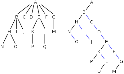
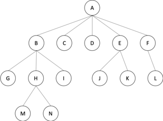
In computer science, a tree is a widely used abstract data type that represents a hierarchical tree structure with a set of connected nodes. Each node in the tree can be connected to many children, but must be connected to exactly one parent, except for the root node, which has no parent. These constraints mean there are no cycles or "loops", and also that each child can be treated like the root node of its own subtree, making recursion a useful technique for tree traversal. In contrast to linear data structures, many trees cannot be represented by relationships between neighboring nodes in a single straight line.

<span class="mw-page-title-main">Smoothsort</span> Comparison-based sorting algorithm

In computer science, smoothsort is a comparison-based sorting algorithm. A variant of heapsort, it was invented and published by Edsger Dijkstra in 1981. Like heapsort, smoothsort is an in-place algorithm with an upper bound of O(n log n) operations (see big O notation), but it is not a stable sort. The advantage of smoothsort is that it comes closer to O(n) time if the input is already sorted to some degree, whereas heapsort averages O(n log n) regardless of the initial sorted state.

<span class="mw-page-title-main">Treap</span>

In computer science, the treap and the randomized binary search tree are two closely related forms of binary search tree data structures that maintain a dynamic set of ordered keys and allow binary searches among the keys. After any sequence of insertions and deletions of keys, the shape of the tree is a random variable with the same probability distribution as a random binary tree; in particular, with high probability its height is proportional to the logarithm of the number of keys, so that each search, insertion, or deletion operation takes logarithmic time to perform.

In computer science, tree traversal is a form of graph traversal and refers to the process of visiting each node in a tree data structure, exactly once. Such traversals are classified by the order in which the nodes are visited. The following algorithms are described for a binary tree, but they may be generalized to other trees as well.

<span class="mw-page-title-main">Rope (data structure)</span> Data structure for storing strings

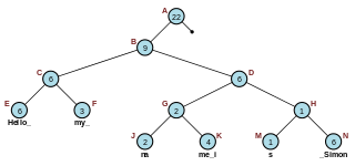
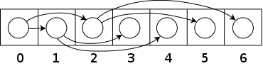
In computer programming, a rope, or cord, is a data structure composed of smaller strings that is used to efficiently store and manipulate a very long string. For example, a text editing program may use a rope to represent the text being edited, so that operations such as insertion, deletion, and random access can be done efficiently.

In computer science, corecursion is a type of operation that is dual to recursion. Whereas recursion works analytically, starting on data further from a base case and breaking it down into smaller data and repeating until one reaches a base case, corecursion works synthetically, starting from a base case and building it up, iteratively producing data further removed from a base case. Put simply, corecursive algorithms use the data that they themselves produce, bit by bit, as they become available, and needed, to produce further bits of data. A similar but distinct concept is generative recursion which may lack a definite "direction" inherent in corecursion and recursion.

In computer science, a scapegoat tree is a self-balancing binary search tree, invented by Arne Andersson in 1989 and again by Igal Galperin and Ronald L. Rivest in 1993. It provides worst-case lookup time and amortized insertion and deletion time.

In computer science, an interval tree is a tree data structure to hold intervals. Specifically, it allows one to efficiently find all intervals that overlap with any given interval or point. It is often used for windowing queries, for instance, to find all roads on a computerized map inside a rectangular viewport, or to find all visible elements inside a three-dimensional scene. A similar data structure is the segment tree.

<i>k</i>-d tree Multidimensional search tree for points in k dimensional space

In computer science, a k-d tree is a space-partitioning data structure for organizing points in a k-dimensional space. K-dimensional is that which concerns exactly k orthogonal axes or a space of any number of dimensions. k-d trees are a useful data structure for several applications, such as:

<i>m</i>-ary tree Tree data structure in which each node has at most m children.

In graph theory, an m-ary tree is an arborescence in which each node has no more than m children. A binary tree is the special case where m = 2, and a ternary tree is another case with m = 3 that limits its children to three.

In computer science, a leftist tree or leftist heap is a priority queue implemented with a variant of a binary heap. Every node x has an s-value which is the distance to the nearest leaf in subtree rooted at x. In contrast to a binary heap, a leftist tree attempts to be very unbalanced. In addition to the heap property, leftist trees are maintained so the right descendant of each node has the lower s-value.

A skew heap is a heap data structure implemented as a binary tree. Skew heaps are advantageous because of their ability to merge more quickly than binary heaps. In contrast with binary heaps, there are no structural constraints, so there is no guarantee that the height of the tree is logarithmic. Only two conditions must be satisfied:

In computer science, weight-balanced binary trees (WBTs) are a type of self-balancing binary search trees that can be used to implement dynamic sets, dictionaries (maps) and sequences. These trees were introduced by Nievergelt and Reingold in the 1970s as trees of bounded balance, or BB[α] trees. Their more common name is due to Knuth.

In computer science, a range tree is an ordered tree data structure to hold a list of points. It allows all points within a given range to be reported efficiently, and is typically used in two or higher dimensions. Range trees were introduced by Jon Louis Bentley in 1979. Similar data structures were discovered independently by Lueker, Lee and Wong, and Willard. The range tree is an alternative to the k-d tree. Compared to k-d trees, range trees offer faster query times of but worse storage of , where n is the number of points stored in the tree, d is the dimension of each point and k is the number of points reported by a given query.

<span class="mw-page-title-main">Cartesian tree</span> Binary tree derived from a sequence of numbers

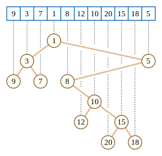
In computer science, a Cartesian tree is a binary tree derived from a sequence of distinct numbers. To construct the Cartesian tree, set its root to be the minimum number in the sequence, and recursively construct its left and right subtrees from the subsequences before and after this number. It is uniquely defined as a min-heap whose symmetric (in-order) traversal returns the original sequence.

In computer science and probability theory, a random binary tree is a binary tree selected at random from some probability distribution on binary trees. Two different distributions are commonly used: binary trees formed by inserting nodes one at a time according to a random permutation, and binary trees chosen from a uniform discrete distribution in which all distinct trees are equally likely. It is also possible to form other distributions, for instance by repeated splitting. Adding and removing nodes directly in a random binary tree will in general disrupt its random structure, but the treap and related randomized binary search tree data structures use the principle of binary trees formed from a random permutation in order to maintain a balanced binary search tree dynamically as nodes are inserted and deleted.

References

Citations

  1. Rowan Garnier; John Taylor (2009). Discrete Mathematics:Proofs, Structures and Applications, Third Edition. CRC Press. p. 620. ISBN   978-1-4398-1280-8.
  2. Steven S Skiena (2009). The Algorithm Design Manual. Springer Science & Business Media. p. 77. ISBN   978-1-84800-070-4.
  3. 1 2 Knuth (1997). The Art Of Computer Programming, Volume 1, 3/E. Pearson Education. p. 363. ISBN   0-201-89683-4.
  4. Iván Flores (1971). Computer programming system/360. Prentice-Hall. p. 39.
  5. Kenneth Rosen (2011). Discrete Mathematics and Its Applications, 7th edition. McGraw-Hill Science. p. 749. ISBN   978-0-07-338309-5.
  6. David R. Mazur (2010). Combinatorics: A Guided Tour. Mathematical Association of America. p. 246. ISBN   978-0-88385-762-5.
  7. 1 2 "Binary tree", Encyclopedia of Mathematics , EMS Press, 2001 [1994] also in print as Michiel Hazewinkel (1997). Encyclopaedia of Mathematics. Supplement I. Springer Science & Business Media. p. 124. ISBN   978-0-7923-4709-5.
  8. L.R. Foulds (1992). Graph Theory Applications. Springer Science & Business Media. p. 32. ISBN   978-0-387-97599-3.
  9. David Makinson (2009). Sets, Logic and Maths for Computing. Springer Science & Business Media. p. 199. ISBN   978-1-84628-845-6.
  10. Jonathan L. Gross (2007). Combinatorial Methods with Computer Applications. CRC Press. p. 248. ISBN   978-1-58488-743-0.
  11. 1 2 Kenneth Rosen (2011). Discrete Mathematics and Its Applications 7th edition. McGraw-Hill Science. pp. 352–353. ISBN   978-0-07-338309-5.
  12. Te Chiang Hu; Man-tak Shing (2002). Combinatorial Algorithms. Courier Dover Publications. p. 162. ISBN   978-0-486-41962-6.
  13. Lih-Hsing Hsu; Cheng-Kuan Lin (2008). Graph Theory and Interconnection Networks. CRC Press. p. 66. ISBN   978-1-4200-4482-9.
  14. J. Flum; M. Grohe (2006). Parameterized Complexity Theory. Springer. p. 245. ISBN   978-3-540-29953-0.
  15. Tamassia, Michael T. Goodrich, Roberto (2011). Algorithm design : foundations, analysis, and Internet examples (2 ed.). New Delhi: Wiley-India. p. 76. ISBN   978-81-265-0986-7.{{cite book}}: CS1 maint: multiple names: authors list (link)
  16. "full binary tree". NIST.
  17. Richard Stanley, Enumerative Combinatorics, volume 2, p.36
  18. "perfect binary tree". NIST.
  19. 1 2 "complete binary tree". NIST.
  20. "almost complete binary tree". Archived from the original on 2016-03-04. Retrieved 2015-12-11.
  21. "nearly complete binary tree" (PDF). Archived (PDF) from the original on 2022-10-09.
  22. Aaron M. Tenenbaum, et al. Data Structures Using C, Prentice Hall, 1990 ISBN   0-13-199746-7
  23. Paul E. Black (ed.), entry for data structure in Dictionary of Algorithms and Data Structures . U.S. National Institute of Standards and Technology. 15 December 2004. Online version Archived December 21, 2010, at the Wayback Machine Accessed 2010-12-19.
  24. Parmar, Anand K. (2020-01-22). "Different Types of Binary Tree with colourful illustrations". Medium. Retrieved 2020-01-24.
  25. Mehta, Dinesh; Sartaj Sahni (2004). Handbook of Data Structures and Applications. Chapman and Hall. ISBN   1-58488-435-5.
  26. D. Samanta (2004). Classic Data Structures. PHI Learning Pvt. Ltd. pp. 264–265. ISBN   978-81-203-1874-8.
  27. Michael L. Scott (2009). Programming Language Pragmatics (3rd ed.). Morgan Kaufmann. p. 347. ISBN   978-0-08-092299-7.
  28. Introduction to algorithms. Cormen, Thomas H., Cormen, Thomas H. (2nd ed.). Cambridge, Mass.: MIT Press. 2001. p. 128. ISBN   0-262-03293-7. OCLC   46792720.{{cite book}}: CS1 maint: others (link)
  29. "Big O Notation Arrays vs. Linked List insertions". Stack Overflow. Retrieved 2023-07-04.
  30. Laakso, Mikko. "Priority Queue and Binary Heap". University of Aalto. Retrieved 2023-10-11.
  31. Demaine, Erik. "6.897: Advanced Data Structures Spring 2003 Lecture 12" (PDF). MIT CSAIL. Archived from the original (PDF) on 24 November 2005. Retrieved 14 April 2022.
  32. 1 2 Dung X. Nguyen (2003). "Binary Tree Structure". rice.edu. Retrieved December 28, 2010.
  33. Wittman, Todd (2015-02-13). "Lecture 18: Tree Traversals" (PDF). Archived from the original (PDF) on 2015-02-13. Retrieved 2023-04-29.

Bibliography