Similarity (network science)

Last updated

Similarity in network analysis occurs when two nodes (or other more elaborate structures) fall in the same equivalence class.

Contents

There are three fundamental approaches to constructing measures of network similarity: structural equivalence, automorphic equivalence, and regular equivalence. [1] There is a hierarchy of the three equivalence concepts: any set of structural equivalences are also automorphic and regular equivalences. Any set of automorphic equivalences are also regular equivalences. Not all regular equivalences are necessarily automorphic or structural; and not all automorphic equivalences are necessarily structural. [2]

Visualizing similarity and distance

Clustering tools

Agglomerative Hierarchical clustering of nodes on the basis of the similarity of their profiles of ties to other nodes provides a joining tree or Dendrogram that visualizes the degree of similarity among cases - and can be used to find approximate equivalence classes. [2]

Multi-dimensional scaling tools

Usually our goal in equivalence analysis is to identify and visualize "classes" or clusters of cases. In using cluster analysis, we are implicitly assuming that the similarity or distance among cases reflects as single underlying dimension. It is possible, however, that there are multiple "aspects" or "dimensions" underlying the observed similarities of cases. Factor or components analysis could be applied to correlations or covariances among cases. Alternatively, multi-dimensional scaling could be used (non-metric for data that are inherently nominal or ordinal; metric for valued). [2]

MDS represents the patterns of similarity or dissimilarity in the tie profiles among the actors (when applied to adjacency or distances) as a "map" in multi-dimensional space. This map lets us see how "close" actors are, whether they "cluster" in multi-dimensional space, and how much variation there is along each dimension. [2]

Structural equivalence

Two vertices of a network are structurally equivalent if they share many of the same neighbors.

Structural equivalence Structural Equivalence.jpg
Structural equivalence

There is no actor who has exactly the same set of ties as actor A, so actor A is in a class by itself. The same is true for actors B, C, D and G. Each of these nodes has a unique set of edges to other nodes. E and F, however, fall in the same structural equivalence class. Each has only one edge; and that tie is to B. Since E and F have exactly the same pattern of edges with all the vertices, they are structurally equivalent. The same is true in the case of H and I. [2]

Structural equivalence is the strongest form of similarity. In many real networks exact equivalence may be rare, and it could be useful to ease the criteria and measure approximate equivalence.

A closely related concept is institutional equivalence: two actors (e.g., firms) are institutionally equivalent if they operate in the same set of institutional fields. [3] While structurally equivalent actors have identical relational patterns or network positions, institutional equivalence captures the similarity of institutional influences that actors experience from being in the same fields, regardless of how similar their network positions are. For example, two banks in Chicago might have very different patterns of ties (e.g., one may be a central node, and the other may be in a peripheral position) such that they are not structural equivalents, but because they both operate in the field of finance and banking and in the same geographically defined field (Chicago), they will be subject to some of the same institutional influences. [3]

Measures for structural equivalence

Cosine similarity

A simple count of common neighbors for two vertices is not on its own a very good measure. One should know the degree of the vertices or how many common neighbors other pairs of vertices has. Cosine similarity takes into account these regards and also allow for the varying degrees of vertices. Salton proposed that we regard the i-th and j-th rows/columns of the adjacency matrix as two vectors and use the cosine of the angle between them as a similarity measure. The cosine similarity of i and j is the number of common neighbors divided by the geometric mean of their degrees. [4]

Its value lies in the range from 0 to 1. The value of 1 indicates that the two vertices have exactly the same neighbors while the value of zero means that they do not have any common neighbors. Cosine similarity is technically undefined if one or both of the nodes has zero degree, but according to the convention we say that cosine similarity is 0 in these cases. [1]

Pearson coefficient

Pearson product-moment correlation coefficient is an alternative method to normalize the count of common neighbors. This method compares the number of common neighbors with the expected value that count would take in a network where vertices are connected randomly. This quantity lies strictly in the range from -1 to 1. [1]

Euclidean distance

Euclidean distance is equal to the number of neighbors that differ between two vertices. It is rather a dissimilarity measure, since it is larger for vertices which differ more. It could be normalized by dividing by its maximum value. The maximum means that there are no common neighbors, in which case the distance is equal to the sum of the degrees of the vertices. [1]

Automorphic equivalence

Formally "Two vertices are automorphically equivalent if all the vertices can be re-labeled to form an isomorphic graph with the labels of u and v interchanged. Two automorphically equivalent vertices share exactly the same label-independent properties." [5]

More intuitively, actors are automorphically equivalent if we can permute the graph in such a way that exchanging the two actors has no effect on the distances among all actors in the graph.

Automorphic equivalence Automorphic equivalence.jpg
Automorphic equivalence

Suppose the graph describes the organizational structure of a company. Actor A is the central headquarter, actors B, C, and D are managers. Actors E, F and H, I are workers at smaller stores; G is the lone worker at another store.

Even though actor B and actor D are not structurally equivalent (they do have the same boss, but not the same workers), they do seem to be "equivalent" in a different sense. Both manager B and D has a boss (in this case, the same boss), and each has two workers. If we swapped them, and also swapped the four workers, all of the distances among all the actors in the network would be exactly identical.

There are actually five automorphic equivalence classes: {A}, {B, D}, {C}, {E, F, H, I}, and {G}. Note that the less strict definition of "equivalence" has reduced the number of classes. [2]

Regular equivalence

Formally, "Two actors are regularly equivalent if they are equally related to equivalent others." In other words, regularly equivalent vertices are vertices that, while they do not necessarily share neighbors, have neighbors who are themselves similar. [5]

Two mothers, for example, are equivalent, because each has a similar pattern of connections with a husband, children, etc. The two mothers do not have ties to the same husband or the same children, so they are not structurally equivalent. Because different mothers may have different numbers of husbands and children, they will not be automorphically equivalent. But they are similar because they have the same relationships with some member or members of another set of actors (who are themselves regarded as equivalent because of the similarity of their ties to a member of the set "mother"). [2]

Regular equivalence Regular equivalence.jpg
Regular equivalence

In the graph there are three regular equivalence classes. The first is actor A; the second is composed of the three actors B, C, and D; the third consists of the remaining five actors E, F, G, H, and I.

The easiest class to see is the five actors across the bottom of the diagram (E, F, G, H, and I). These actors are regularly equivalent to one another because:

  1. they have no tie with any actor in the first class (that is, with actor A) and
  2. each has a tie with an actor in the second class (either B or C or D).

Each of the five actors, then, has an identical pattern of ties with actors in the other classes.

Actors B, C, and D form a class similarly. B and D actually have ties with two members of the third class, whereas actor C has a tie to only one member of the third class, but this doesn't matter, as there is a tie to some member of the third class.

Actor A is in a class by itself, defined by:

  1. a tie to at least one member of class two and
  2. no tie to any member of class three. [2]

See also

Related Research Articles

In graph theory, a planar graph is a graph that can be embedded in the plane, i.e., it can be drawn on the plane in such a way that its edges intersect only at their endpoints. In other words, it can be drawn in such a way that no edges cross each other. Such a drawing is called a plane graph or planar embedding of the graph. A plane graph can be defined as a planar graph with a mapping from every node to a point on a plane, and from every edge to a plane curve on that plane, such that the extreme points of each curve are the points mapped from its end nodes, and all curves are disjoint except on their extreme points.

Bipartite graph Graph in which every vertex is connected to at least one other

In the mathematical field of graph theory, a bipartite graph is a graph whose vertices can be divided into two disjoint and independent sets and such that every edge connects a vertex in to one in . Vertex sets and are usually called the parts of the graph. Equivalently, a bipartite graph is a graph that does not contain any odd-length cycles.

Graph isomorphism Bijection between the vertex set of two graphs

In graph theory, an isomorphism of graphsG and H is a bijection between the vertex sets of G and H

This is a glossary of graph theory. Graph theory is the study of graphs, systems of nodes or vertices connected in pairs by lines or edges.

In mathematics, computer science and especially graph theory, a distance matrix is a square matrix containing the distances, taken pairwise, between the elements of a set. Depending upon the application involved, the distance being used to define this matrix may or may not be a metric. If there are N elements, this matrix will have size N×N. In graph-theoretic applications the elements are more often referred to as points, nodes or vertices.

Bridge (graph theory) Edge in node-link graph whose removal would disconnect the graph

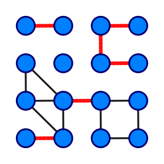
In graph theory, a bridge, isthmus, cut-edge, or cut arc is an edge of a graph whose deletion increases the graph's number of connected components. Equivalently, an edge is a bridge if and only if it is not contained in any cycle. For a connected graph, a bridge can uniquely determine a cut. A graph is said to be bridgeless or isthmus-free if it contains no bridges.

Centrality

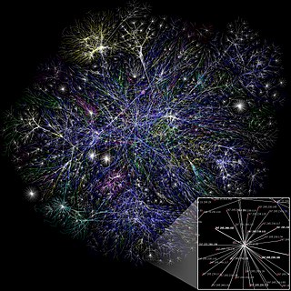
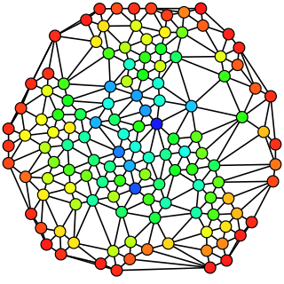
In graph theory and network analysis, indicators of centrality assign numbers or rankings to nodes within a graph corresponding to their network position. Applications include identifying the most influential person(s) in a social network, key infrastructure nodes in the Internet or urban networks, super-spreaders of disease, and brain networks. Centrality concepts were first developed in social network analysis, and many of the terms used to measure centrality reflect their sociological origin.

Connectivity (graph theory) Basic concept of graph theory

In mathematics and computer science, connectivity is one of the basic concepts of graph theory: it asks for the minimum number of elements that need to be removed to separate the remaining nodes into two or more isolated subgraphs. It is closely related to the theory of network flow problems. The connectivity of a graph is an important measure of its resilience as a network.

Signed graph

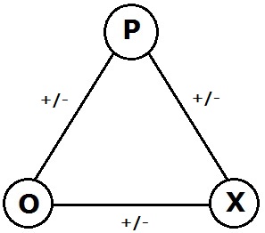
In the area of graph theory in mathematics, a signed graph is a graph in which each edge has a positive or negative sign.

In constraint satisfaction, a decomposition method translates a constraint satisfaction problem into another constraint satisfaction problem that is binary and acyclic. Decomposition methods work by grouping variables into sets, and solving a subproblem for each set. These translations are done because solving binary acyclic problems is a tractable problem.

Assortativity Tendency for similar nodes to be connected

Assortativity, or assortative mixing is a preference for a network's nodes to attach to others that are similar in some way. Though the specific measure of similarity may vary, network theorists often examine assortativity in terms of a node's degree. The addition of this characteristic to network models more closely approximates the behaviors of many real world networks.

Triadic closure

Triadic closure is a concept in social network theory, first suggested by German sociologist Georg Simmel in his 1908 book Soziologie [Sociology: Investigations on the Forms of Sociation]. Triadic closure is the property among three nodes A, B, and C, that if the connections A-B and B-C exist, there is a tendency for the new connection A-C to be formed. Triadic closure can be used to understand and predict the growth of networks, although it is only one of many mechanisms by which new connections are formed in complex networks.

Median graph

In graph theory, a division of mathematics, a median graph is an undirected graph in which every three vertices a, b, and c have a unique median: a vertex m(a,b,c) that belongs to shortest paths between each pair of a, b, and c.

Separable permutation

In combinatorial mathematics, a separable permutation is a permutation that can be obtained from the trivial permutation 1 by direct sums and skew sums. Separable permutations may be characterized by the forbidden permutation patterns 2413 and 3142; they are also the permutations whose permutation graphs are cographs and the permutations that realize the series-parallel partial orders. It is possible to test in polynomial time whether a given separable permutation is a pattern in a larger permutation, or to find the longest common subpattern of two separable permutations.

In graph theory, a partial cube is a graph that is isometric to a subgraph of a hypercube. In other words, a partial cube can be identified with a subgraph of a hypercube in such a way that the distance between any two vertices in the partial cube is the same as the distance between those vertices in the hypercube. Equivalently, a partial cube is a graph whose vertices can be labeled with bit strings of equal length in such a way that the distance between two vertices in the graph is equal to the Hamming distance between their labels. Such a labeling is called a Hamming labeling; it represents an isometric embedding of the partial cube into a hypercube.

Betweenness centrality

In graph theory, betweenness centrality is a measure of centrality in a graph based on shortest paths. For every pair of vertices in a connected graph, there exists at least one shortest path between the vertices such that either the number of edges that the path passes through or the sum of the weights of the edges is minimized. The betweenness centrality for each vertex is the number of these shortest paths that pass through the vertex.

In the mathematics of infinite graphs, an end of a graph represents, intuitively, a direction in which the graph extends to infinity. Ends may be formalized mathematically as equivalence classes of infinite paths, as havens describing strategies for pursuit-evasion games on the graph, or as topological ends of topological spaces associated with the graph.

In discrete mathematics and theoretical computer science, the rotation distance between two binary trees with the same number of nodes is the minimum number of tree rotations needed to reconfigure one tree into another. Because of a combinatorial equivalence between binary trees and triangulations of convex polygons, rotation distance is equivalent to the flip distance for triangulations of convex polygons.

In network theory, link prediction is the problem of predicting the existence of a link between two entities in a network. Examples of link prediction include predicting friendship links among users in a social network, predicting co-authorship links in a citation network, and predicting interactions between genes and proteins in a biological network. Link prediction can also have a temporal aspect, where, given a snapshot of the set of links at time , the goal is to predict the links at time . Link prediction is widely applicable. In e-commerce, link prediction is often a subtask for recommending items to users. In the curation of citation databases, it can be used for record deduplication. In bioinformatics, it has been used to predict protein-protein interactions (PPI). It is also used to identify hidden groups of terrorists and criminals in security related applications.

Blockmodeling refers to a set or a coherent framework, that is used for analyzing social structure and also for setting procedure(s) for partitioning (clustering) social network's units, based on specific patterns, which form a distinctive structure through interconnectivity. It is primarily used in statistics, machine learning, and network science.

References

  1. 1 2 3 4 Newman, M.E.J. 2010. Networks: An Introduction. Oxford, UK: Oxford University Press.
  2. 1 2 3 4 5 6 7 8 Hanneman, Robert A. and Mark Riddle. 2005. Introduction to social network methods. Riverside, CA: University of California, Riverside ( published in digital form at http://faculty.ucr.edu/~hanneman/ )
  3. 1 2 Marquis, Christopher; Tilcsik, András (2016-10-01). "Institutional Equivalence: How Industry and Community Peers Influence Corporate Philanthropy". Organization Science. 27 (5): 1325–1341. doi:10.1287/orsc.2016.1083. hdl: 1813/44734 . ISSN   1047-7039.
  4. Salton G., Automatic Text Processing: The Transformation, Analysis and Retrieval of Information by Computer, Addison-Wesley, Reading, MA (1989)
  5. 1 2 Borgatti, Steven, Martin Everett, and Linton Freeman. 1992. UCINET IV Version 1.0 User's Guide. Columbia, SC: Analytic Technologies.