2D adaptive filters

Last updated October 05, 2024

A two-dimensional (2D) adaptive filter is very much like a one-dimensional adaptive filter in that it is a linear system whose parameters are adaptively updated throughout the process, according to some optimization approach. The main difference between 1D and 2D adaptive filters is that the former usually take as inputs signals with respect to time, what implies in causality constraints, while the latter handles signals with 2 dimensions, like x-y coordinates in the space domain, which are usually non-causal. Moreover, just like 1D filters, most 2D adaptive filters are digital filters, because of the complex and iterative nature of the algorithms.

Motivation

The topic of 2D adaptive filters is very important in electrical engineering and signal processing since these filters have the ability to take into account the nonstationary statistical properties of 2D signals. Adaptive filters find applications in areas such as Noise cancellation, Signal prediction, Equalization and Echo cancellation. Examples of applications of 2D adaptive filters include Image Denoising,^[1] Motion Tracking,^[2] OFDM channel estimation,^[3] magnetic recording equalization ^[4]

Example Application

2D Adaptive Filters can be used to identify systems. The system function of the unknown system is given by $P(z_{1},z_{2})$ , and $H(z_{1},z_{2})$ is the system function of the 2D adaptive filter when its output comes to steady. The error signal $e(n_{1},n_{2})$ between the unknown system output, $d(n_{1},n_{2})$ , and the adaptive filter output, $y(n_{1},n_{2})$ , is minimized if the unknown system and known 2D adaptive filter have the same input, and if the resulting outputs are similar. Then, it can be shown that $P(z_{1},z_{2})$ can be represented by $H(z_{1},z_{2})$ . $H(z_{1},z_{2})$ is known as the system identification model of the unknown system.

Problem Statement

General Block Diagram for a 2D Adaptive Filter. Adaptivefilter1.png — General Block Diagram for a 2D Adaptive Filter.

In digital signal processing, any linear shift invariant system can be represented by the convolution of the signal with the filter's impulse response, given by the expression:

$y(n_{1},n_{2})=\sum _{m_{1}}\sum _{m_{2}}w(m_{1},m_{2})x(n_{1}-m_{1},n_{2}-m_{2})$

If this system is to model a desired response $d(n_{1},n_{2})$ , the adaptive system can be obtained by continuously adjusting the weight values according to some cost function $F[e(n_{1},n_{2})]$ that evaluates the error between the two responses.

$e(n_{1},n_{2})=d(n_{1},n_{2})-y(n_{1},n_{2})$
$w_{j+1}(n_{1},n_{2})=w_{j}(n_{1},n_{2})+F[e(n_{1},n_{2})]$

Approaches

2D Least Mean Square FIR Adaptive Filters

Least mean square (LMS) Adaptive Filters^[5] use the most common error measure method, the mean square error. The 2D LMS Adaptive filters are derived from the 1D LMS adaptive filters main method which minimizes the output mean square value by adjusting coefficients of the filter. The filter has the primary 2D input signal d and the reference input signal x. The primary input signal d consists of the ideal signal and noise component. The filter is an N by N causal FIR filter with impulse response $w$ . Then we can get the filter output given by

$y(n_{1},n_{2})=\sum _{m_{1}=0}^{N-1}\sum _{m_{2}=0}^{N-1}w_{j}(m_{1},m_{2})x(n_{1}-m_{1},n_{2}-m_{2})$

where j is the iteration number for adaptive filters.

The error signal $e_{j}$ at the j-th iteration is defined as

$e_{j}=d(n_{1},n_{2})-\sum _{m_{1}=0}^{N-1}\sum _{m_{2}=0}^{N-1}w_{j}(m_{1},m_{2})x(n_{1}-m_{1},n_{2}-m_{2})$

The weight matrix at the next iteration is equal to the present weight matrix plus a change proportional to the negative gradient of the mean square error. For the two-dimensional LMS adaptive filter, the filter coefficients are updated as follows:

$w_{j+1}(n_{1},n_{2})=w_{j}(n_{1},n_{2})+2\mu e_{j}x(n_{1},n_{2})$

where $\mu$ is the scaler multiplier controlling which can control the rate of convergence and filter stability.

Advantages: The TDLMS adaptive filter can be implemented without any form of matrix operations or any averaging or differentiation. The algorithm convergence does not depend on the initial conditions and it will converge for any arbitrarily initial value, hence, it provides good performance in nonstationary images.

Disadvantages: The exact values of the expectations of the TDLMS adaptive filter will not converges to a fixed value, if we need to maintain its tracking ability. Therefore, the design choice of μ depends on the particular application and it involves a tradeoff between the convergence speed, tracking ability, and steady-state MSE.

2D Least Mean Square IIR Adaptive Filters

For a two-dimensional LMS IIR Adaptive filter, its basic idea is the same as 2D LMS FIR Adaptive Filters, except we are using an IIR filter, which can reduce the filter order requirements.^[6] The two-dimensional IIR filter`s difference equation can be written as

$y(n_{1},n_{2})=\sum _{m_{1}=0}^{M_{1}}\sum _{m_{2}=0}^{M_{2}}a(m_{1},m_{2})x(n_{1}-m_{1},n_{2}-m_{2})-{\sum _{m_{1}=0}^{L_{1}}\sum _{m_{2}=0}^{L_{2}}}_{(m_{1},m_{2})\neq (0,0)}b(m_{1},m_{2})y(n_{1}-m_{1},n_{2}-m_{2})$

where $y(n_{1},n_{2})$ and $x(n_{1},n_{2})$ are, respectively, the output and input of the adaptive filter. $b(m_{1},m_{2})$ and $a(m_{1},m_{2})$ are the masks of the filter`s input and output. The error signal is given by

$e(n_{1},n_{2})=d(n_{1},n_{2})-y(n_{1},n_{2})$

where $d(n_{1},n_{2})$ is the primary output signal.

The mean square error $E\{e^{2}(n_{1},n_{2})\}$ is minimized by updating the filter weights in a manner to converge to the optimum filter weight.

Advantages: IIR filters can satisfy the prescribed frequency response because it can reduce the filter`s order requirements.

Disadvantages: The performance surfaces of adaptive LMS IIR Adaptive filters are nonquadratic and may have local minima. Meanwhile, adaptive IIR filters may become unstable during the adaptation, thus some kind of stability monitoring is needed.

Recursive least square adaptive filters

2D Recursive Least Square Adaptive Filters^[7] can be developed by applying 1D recursive least squares filters along both horizontal and vertical directions. The RLS adaptive is an algorithm which finds the filter coefficients recursively to minimize the weighted least squares cost function. The RLS algorithm is different to the least mean squares algorithm which aim to reduce the mean square error, its input signal is considered deterministic. For this reason, the RLS algorithm has fast convergence characteristic.

Advantages: The RLS algorithm has fast convergence property. The accuracy of image denoising based on RLS algorithm is better than 2D LMS adaptive filters.

Disadvantages: The RLS algorithm needs a large amount of computations, especially in two-dimensional and multidimensional case.

Lexicographic Ordering

One convenient approach to implement 2D Adaptive Filters is to transform the 2D problem into a 1D problem by lexicographic ordering.^[5] This simplifies the implementation and makes it possible to benefit from the extensive literature that is available for 1D adaptive filters and utilize all of the existing 1D algorithms.

McClellan Transformations

McClellan transformations^[8] can be used to transform a 1D filter design into a 2D filter design by using a transformation function. This theory allows the design of 2D adaptive filters ^[9] out of existing 1D prototype filters. Compared to the direct approach, this system has the advantages of a lower computational complexity and a faster convergence rate. However, in order to work properly, it needs some a priori information about the system to correctly select the transformation function parameters, making the system pre-constrained.

Block Diagonal 2D Adaptive Filters

Block Diagonal 2D Adaptive Filters is an alternative approach ^[10] that scans the signal through blocks and applies weight adjustments for each block, instead of for each sample as in the traditional adaptive filters. The advantage of this kind of system is that it takes into account signal correlations along both dimensions. On the other hand, it assumes a higher local stationarity of the signal.

Related Research Articles

In signal processing, a digital filter is a system that performs mathematical operations on a sampled, discrete-time signal to reduce or enhance certain aspects of that signal. This is in contrast to the other major type of electronic filter, the analog filter, which is typically an electronic circuit operating on continuous-time analog signals.

A wavelet is a wave-like oscillation with an amplitude that begins at zero, increases or decreases, and then returns to zero one or more times. Wavelets are termed a "brief oscillation". A taxonomy of wavelets has been established, based on the number and direction of its pulses. Wavelets are imbued with specific properties that make them useful for signal processing.

An adaptive filter is a system with a linear filter that has a transfer function controlled by variable parameters and a means to adjust those parameters according to an optimization algorithm. Because of the complexity of the optimization algorithms, almost all adaptive filters are digital filters. Adaptive filters are required for some applications because some parameters of the desired processing operation are not known in advance or are changing. The closed loop adaptive filter uses feedback in the form of an error signal to refine its transfer function.

In signal processing, a finite impulse response (FIR) filter is a filter whose impulse response is of finite duration, because it settles to zero in finite time. This is in contrast to infinite impulse response (IIR) filters, which may have internal feedback and may continue to respond indefinitely.

In signal processing, specifically control theory, bounded-input, bounded-output (BIBO) stability is a form of stability for signals and systems that take inputs. If a system is BIBO stable, then the output will be bounded for every input to the system that is bounded.

Stochastic gradient descent is an iterative method for optimizing an objective function with suitable smoothness properties. It can be regarded as a stochastic approximation of gradient descent optimization, since it replaces the actual gradient by an estimate thereof. Especially in high-dimensional optimization problems this reduces the very high computational burden, achieving faster iterations in exchange for a lower convergence rate.

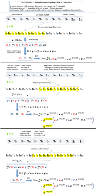
In signal processing, a filter bank is an array of bandpass filters that separates the input signal into multiple components, each one carrying a sub-band of the original signal. One application of a filter bank is a graphic equalizer, which can attenuate the components differently and recombine them into a modified version of the original signal. The process of decomposition performed by the filter bank is called analysis ; the output of analysis is referred to as a subband signal with as many subbands as there are filters in the filter bank. The reconstruction process is called synthesis, meaning reconstitution of a complete signal resulting from the filtering process.

Least mean squares (LMS) algorithms are a class of adaptive filter used to mimic a desired filter by finding the filter coefficients that relate to producing the least mean square of the error signal. It is a stochastic gradient descent method in that the filter is only adapted based on the error at the current time. It was invented in 1960 by Stanford University professor Bernard Widrow and his first Ph.D. student, Ted Hoff, based on their research in single-layer neural networks (ADALINE). Specifically, they used gradient descent to train ADALINE to recognize patterns, and called the algorithm "delta rule". They then applied the rule to filters, resulting in the LMS algorithm.

Recursive least squares (RLS) is an adaptive filter algorithm that recursively finds the coefficients that minimize a weighted linear least squares cost function relating to the input signals. This approach is in contrast to other algorithms such as the least mean squares (LMS) that aim to reduce the mean square error. In the derivation of the RLS, the input signals are considered deterministic, while for the LMS and similar algorithms they are considered stochastic. Compared to most of its competitors, the RLS exhibits extremely fast convergence. However, this benefit comes at the cost of high computational complexity.

In mathematics, a wavelet series is a representation of a square-integrable function by a certain orthonormal series generated by a wavelet. This article provides a formal, mathematical definition of an orthonormal wavelet and of the integral wavelet transform.

Space-time adaptive processing (STAP) is a signal processing technique most commonly used in radar systems. It involves adaptive array processing algorithms to aid in target detection. Radar signal processing benefits from STAP in areas where interference is a problem. Through careful application of STAP, it is possible to achieve order-of-magnitude sensitivity improvements in target detection.

Mean shift is a non-parametric feature-space mathematical analysis technique for locating the maxima of a density function, a so-called mode-seeking algorithm. Application domains include cluster analysis in computer vision and image processing.

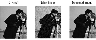
In signal processing, particularly image processing, total variation denoising, also known as total variation regularization or total variation filtering, is a noise removal process (filter). It is based on the principle that signals with excessive and possibly spurious detail have high total variation, that is, the integral of the image gradient magnitude is high. According to this principle, reducing the total variation of the signal—subject to it being a close match to the original signal—removes unwanted detail whilst preserving important details such as edges. The concept was pioneered by L. I. Rudin, S. Osher, and E. Fatemi in 1992 and so is today known as the ROF model.

Two dimensional filters have seen substantial development effort due to their importance and high applicability across several domains. In the 2-D case the situation is quite different from the 1-D case, because the multi-dimensional polynomials cannot in general be factored. This means that an arbitrary transfer function cannot generally be manipulated into a form required by a particular implementation. The input-output relationship of a 2-D IIR filter obeys a constant-coefficient linear partial difference equation from which the value of an output sample can be computed using the input samples and previously computed output samples. Because the values of the output samples are fed back, the 2-D filter, like its 1-D counterpart, can be unstable.

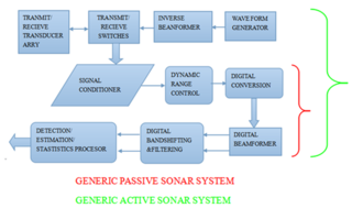
Sonar systems are generally used underwater for range finding and detection. Active sonar emits an acoustic signal, or pulse of sound, into the water. The sound bounces off the target object and returns an echo to the sonar transducer. Unlike active sonar, passive sonar does not emit its own signal, which is an advantage for military vessels. But passive sonar cannot measure the range of an object unless it is used in conjunction with other passive listening devices. Multiple passive sonar devices must be used for triangulation of a sound source. No matter whether active sonar or passive sonar, the information included in the reflected signal can not be used without technical signal processing. To extract the useful information from the mixed signal, some steps are taken to transfer the raw acoustic data.

This article provides a short survey of the concepts, principles and applications of Multirate filter banks and Multidimensional Directional filter banks.

In signal processing, multidimensional discrete convolution refers to the mathematical operation between two functions f and g on an n-dimensional lattice that produces a third function, also of n-dimensions. Multidimensional discrete convolution is the discrete analog of the multidimensional convolution of functions on Euclidean space. It is also a special case of convolution on groups when the group is the group of n-tuples of integers.

In signal processing, nonlinear multidimensional signal processing (NMSP) covers all signal processing using nonlinear multidimensional signals and systems. Nonlinear multidimensional signal processing is a subset of signal processing (multidimensional signal processing). Nonlinear multi-dimensional systems can be used in a broad range such as imaging, teletraffic, communications, hydrology, geology, and economics. Nonlinear systems cannot be treated as linear systems, using Fourier transformation and wavelet analysis. Nonlinear systems will have chaotic behavior, limit cycle, steady state, bifurcation, multi-stability and so on. Nonlinear systems do not have a canonical representation, like impulse response for linear systems. But there are some efforts to characterize nonlinear systems, such as Volterra and Wiener series using polynomial integrals as the use of those methods naturally extend the signal into multi-dimensions. Another example is the Empirical mode decomposition method using Hilbert transform instead of Fourier Transform for nonlinear multi-dimensional systems. This method is an empirical method and can be directly applied to data sets. Multi-dimensional nonlinear filters (MDNF) are also an important part of NMSP, MDNF are mainly used to filter noise in real data. There are nonlinear-type hybrid filters used in color image processing, nonlinear edge-preserving filters use in magnetic resonance image restoration. Those filters use both temporal and spatial information and combine the maximum likelihood estimate with the spatial smoothing algorithm.

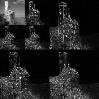
In signal processing, multidimensional empirical mode decomposition is an extension of the one-dimensional (1-D) EMD algorithm to a signal encompassing multiple dimensions. The Hilbert–Huang empirical mode decomposition (EMD) process decomposes a signal into intrinsic mode functions combined with the Hilbert spectral analysis, known as the Hilbert–Huang transform (HHT). The multidimensional EMD extends the 1-D EMD algorithm into multiple-dimensional signals. This decomposition can be applied to image processing, audio signal processing, and various other multidimensional signals.

Parallelmultidimensionaldigitalsignal processing (mD-DSP) is defined as the application of parallel programming and multiprocessing to digital signal processing techniques to process digital signals that have more than a single dimension. The use of mD-DSP is fundamental to many application areas such as digital image and video processing, medical imaging, geophysical signal analysis, sonar, radar, lidar, array processing, computer vision, computational photography, and augmented and virtual reality. However, as the number of dimensions of a signal increases the computational complexity to operate on the signal increases rapidly. This relationship between the number of dimensions and the amount of complexity, related to both time and space, as studied in the field of algorithm analysis, is analogues to the concept of the curse of dimensionality. This large complexity generally results in an extremely long execution run-time of a given mD-DSP application rendering its usage to become impractical for many applications; especially for real-time applications. This long run-time is the primary motivation of applying parallel algorithmic techniques to mD-DSP problems.

References

↑ Abadi, M. Shams Esfand, and S. Nikbakht. "Image denoising with two-dimensional adaptive filter algorithms." Iranian Journal of Electrical & Electronic Engineering 7.2 (2011).
↑ Trimeche, Mejdi. "Hierarchical Motion Estimation Using Recursive LMS Filters." (2007).
↑ Hou, Xiaolin, et al. "On two-dimensional adaptive channel estimation in OFDM systems." Vehicular Technology Conference, 2004. VTC2004-Fall. 2004 IEEE 60th. Vol. 1. IEEE, 2004.
↑ Kumar, P. Sarath, and Sumit Roy. "Two-dimensional equalization: Theory and applications to high density magnetic recording." Communications, IEEE Transactions on 42.234 (1994): 386-395.
1 2 Mohiy M.Hadhoud and David W.Thomas. "Two-Dimensional Adaptive LMS (TDLMS) Algorithm." IEEE Transactions on Circuits And Systems, Vol 35, No.5, May 1988.
↑ Alfredo C. Tan and Sheng-Tsal Chen, "Two-Dimensional Adaptive LMS IIR Filter." Circuits and Systems, 1993., ISCAS '93, 1993 IEEE International Symposium on Date 3–6 May 1993.
↑ Mitsuji Muneyasu, Eiji Uemoto and Takao Hinamoto. "A Novel 2-D Adaptive Filter Based On The 1-D RLS Algorithm." Circuits and Systems, 1997. ISCAS '97., Proceedings of 1997 IEEE International Symposium on 9-12 June 1997
↑ McClellan, James H. "The design of two-dimensional digital filters by transformations." Proc. 7th Annu. Princeton Conf. Information Sciences and Systems. 1973.
↑ Jenkins, W. K., and R. P. Faust. "A constrained two-dimensional adaptive digital filter with reduced computational complexity." Circuits and Systems, 1988., IEEE International Symposium on. IEEE, 1988.
↑ Azimi-Sadjadi, Mahmood R., and Hongye Pan. "Two-dimensional block diagonal LMS adaptive filtering Archived 2018-12-21 at the Wayback Machine ." Signal Processing, IEEE Transactions on 42.9 (1994): 2420-2429.

This page is based on this Wikipedia article
Text is available under the CC BY-SA 4.0 license; additional terms may apply.
Images, videos and audio are available under their respective licenses.

[1] Abadi, M. Shams Esfand, and S. Nikbakht. "Image denoising with two-dimensional adaptive filter algorithms." Iranian Journal of Electrical & Electronic Engineering 7.2 (2011).

[2] Trimeche, Mejdi. "Hierarchical Motion Estimation Using Recursive LMS Filters." (2007).

[3] Hou, Xiaolin, et al. "On two-dimensional adaptive channel estimation in OFDM systems." Vehicular Technology Conference, 2004. VTC2004-Fall. 2004 IEEE 60th. Vol. 1. IEEE, 2004.

[4] Kumar, P. Sarath, and Sumit Roy. "Two-dimensional equalization: Theory and applications to high density magnetic recording." Communications, IEEE Transactions on 42.234 (1994): 386-395.

[Mohiy-5] 1 2 Mohiy M.Hadhoud and David W.Thomas. "Two-Dimensional Adaptive LMS (TDLMS) Algorithm." IEEE Transactions on Circuits And Systems, Vol 35, No.5, May 1988.

[6] Alfredo C. Tan and Sheng-Tsal Chen, "Two-Dimensional Adaptive LMS IIR Filter." Circuits and Systems, 1993., ISCAS '93, 1993 IEEE International Symposium on Date 3–6 May 1993.

[7] Mitsuji Muneyasu, Eiji Uemoto and Takao Hinamoto. "A Novel 2-D Adaptive Filter Based On The 1-D RLS Algorithm." Circuits and Systems, 1997. ISCAS '97., Proceedings of 1997 IEEE International Symposium on 9-12 June 1997

[8] McClellan, James H. "The design of two-dimensional digital filters by transformations." Proc. 7th Annu. Princeton Conf. Information Sciences and Systems. 1973.

[9] Jenkins, W. K., and R. P. Faust. "A constrained two-dimensional adaptive digital filter with reduced computational complexity." Circuits and Systems, 1988., IEEE International Symposium on. IEEE, 1988.

[10] Azimi-Sadjadi, Mahmood R., and Hongye Pan. "Two-dimensional block diagonal LMS adaptive filtering Archived 2018-12-21 at the Wayback Machine ." Signal Processing, IEEE Transactions on 42.9 (1994): 2420-2429.

[1]

[2]

[3]

[4]

[5]

[6]

[7]

[8]

[9]

[10]