A finite difference is a mathematical expression of the form f (x + b) − f (x + a). If a finite difference is divided by b − a, one gets a difference quotient. The approximation of derivatives by finite differences plays a central role in finite difference methods for the numerical solution of differential equations, especially boundary value problems.

In numerical analysis, the Runge–Kutta methods are a family of implicit and explicit iterative methods, which include the Euler method, used in temporal discretization for the approximate solutions of simultaneous nonlinear equations. These methods were developed around 1900 by the German mathematicians Carl Runge and Wilhelm Kutta.

Numerical methods for ordinary differential equations are methods used to find numerical approximations to the solutions of ordinary differential equations (ODEs). Their use is also known as "numerical integration", although this term can also refer to the computation of integrals.
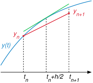
In numerical analysis, a branch of applied mathematics, the midpoint method is a one-step method for numerically solving the differential equation,
In electrical engineering, a differential-algebraic system of equations (DAEs) is a system of equations that either contains differential equations and algebraic equations, or is equivalent to such a system. In mathematics these are examples of ``differential algebraic varieties and correspond to ideals in differential polynomial rings (see the article on differential algebra for the algebraic setup.
Linear multistep methods are used for the numerical solution of ordinary differential equations. Conceptually, a numerical method starts from an initial point and then takes a short step forward in time to find the next solution point. The process continues with subsequent steps to map out the solution. Single-step methods refer to only one previous point and its derivative to determine the current value. Methods such as Runge–Kutta take some intermediate steps to obtain a higher order method, but then discard all previous information before taking a second step. Multistep methods attempt to gain efficiency by keeping and using the information from previous steps rather than discarding it. Consequently, multistep methods refer to several previous points and derivative values. In the case of linear multistep methods, a linear combination of the previous points and derivative values is used.
In mathematics, a stiff equation is a differential equation for which certain numerical methods for solving the equation are numerically unstable, unless the step size is taken to be extremely small. It has proven difficult to formulate a precise definition of stiffness, but the main idea is that the equation includes some terms that can lead to rapid variation in the solution.
In mathematics and computational science, the Euler method is a first-order numerical procedure for solving ordinary differential equations (ODEs) with a given initial value. It is the most basic explicit method for numerical integration of ordinary differential equations and is the simplest Runge–Kutta method. The Euler method is named after Leonhard Euler, who treated it in his book Institutionum calculi integralis.
In numerical analysis and scientific computing, the backward Euler method is one of the most basic numerical methods for the solution of ordinary differential equations. It is similar to the (standard) Euler method, but differs in that it is an implicit method. The backward Euler method has error of order one in time.
In numerical analysis, finite-difference methods (FDM) are a class of numerical techniques for solving differential equations by approximating derivatives with finite differences. Both the spatial domain and time interval are discretized, or broken into a finite number of steps, and the value of the solution at these discrete points is approximated by solving algebraic equations containing finite differences and values from nearby points.
The Kantorovich theorem, or Newton–Kantorovich theorem, is a mathematical statement on the semi-local convergence of Newton's method. It was first stated by Leonid Kantorovich in 1948. It is similar to the form of the Banach fixed-point theorem, although it states existence and uniqueness of a zero rather than a fixed point.
In mathematics and computational science, Heun's method may refer to the improved or modified Euler's method, or a similar two-stage Runge–Kutta method. It is named after Karl Heun and is a numerical procedure for solving ordinary differential equations (ODEs) with a given initial value. Both variants can be seen as extensions of the Euler method into two-stage second-order Runge–Kutta methods.
In numerical analysis, predictor–corrector methods belong to a class of algorithms designed to integrate ordinary differential equations – to find an unknown function that satisfies a given differential equation. All such algorithms proceed in two steps:
- The initial, "prediction" step, starts from a function fitted to the function-values and derivative-values at a preceding set of points to extrapolate ("anticipate") this function's value at a subsequent, new point.
- The next, "corrector" step refines the initial approximation by using the predicted value of the function and another method to interpolate that unknown function's value at the same subsequent point.
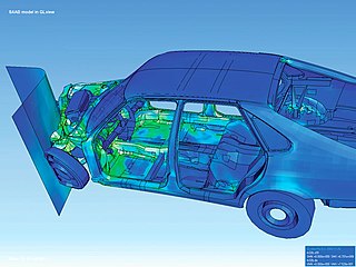
The finite element method (FEM) is a popular method for numerically solving differential equations arising in engineering and mathematical modeling. Typical problem areas of interest include the traditional fields of structural analysis, heat transfer, fluid flow, mass transport, and electromagnetic potential.
The Bogacki–Shampine method is a method for the numerical solution of ordinary differential equations, that was proposed by Przemysław Bogacki and Lawrence F. Shampine in 1989. The Bogacki–Shampine method is a Runge–Kutta method of order three with four stages with the First Same As Last (FSAL) property, so that it uses approximately three function evaluations per step. It has an embedded second-order method which can be used to implement adaptive step size. The Bogacki–Shampine method is implemented in the ode3 for fixed step solver and ode23 for a variable step solver function in MATLAB.
Truncation errors in numerical integration are of two kinds:
In numerical analysis and scientific computing, the trapezoidal rule is a numerical method to solve ordinary differential equations derived from the trapezoidal rule for computing integrals. The trapezoidal rule is an implicit second-order method, which can be considered as both a Runge–Kutta method and a linear multistep method.
In the fields of dynamical systems and control theory, a fractional-order system is a dynamical system that can be modeled by a fractional differential equation containing derivatives of non-integer order. Such systems are said to have fractional dynamics. Derivatives and integrals of fractional orders are used to describe objects that can be characterized by power-law nonlocality, power-law long-range dependence or fractal properties. Fractional-order systems are useful in studying the anomalous behavior of dynamical systems in physics, electrochemistry, biology, viscoelasticity and chaotic systems.
General linear methods (GLMs) are a large class of numerical methods used to obtain numerical solutions to ordinary differential equations. They include multistage Runge–Kutta methods that use intermediate collocation points, as well as linear multistep methods that save a finite time history of the solution. John C. Butcher originally coined this term for these methods, and has written a series of review papers a book chapter and a textbook on the topic. His collaborator, Zdzislaw Jackiewicz also has an extensive textbook on the topic. The original class of methods were originally proposed by Butcher (1965), Gear (1965) and Gragg and Stetter (1964).
Zero-stability, also known as D-stability in honor of Germund Dahlquist, refers to the stability of a numerical scheme applied to the simple initial value problem .


 BDF1
BDF1 BDF2
BDF2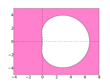 BDF3
BDF3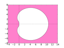 BDF4
BDF4 BDF5
BDF5 BDF6
BDF6


