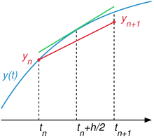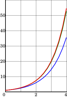
In numerical analysis, the Runge–Kutta methods are a family of implicit and explicit iterative methods, which include the Euler method, used in temporal discretization for the approximate solutions of simultaneous nonlinear equations. These methods were developed around 1900 by the German mathematicians Carl Runge and Wilhelm Kutta.

Numerical methods for ordinary differential equations are methods used to find numerical approximations to the solutions of ordinary differential equations (ODEs). Their use is also known as "numerical integration", although this term can also refer to the computation of integrals.
Linear multistep methods are used for the numerical solution of ordinary differential equations. Conceptually, a numerical method starts from an initial point and then takes a short step forward in time to find the next solution point. The process continues with subsequent steps to map out the solution. Single-step methods refer to only one previous point and its derivative to determine the current value. Methods such as Runge–Kutta take some intermediate steps to obtain a higher order method, but then discard all previous information before taking a second step. Multistep methods attempt to gain efficiency by keeping and using the information from previous steps rather than discarding it. Consequently, multistep methods refer to several previous points and derivative values. In the case of linear multistep methods, a linear combination of the previous points and derivative values is used.
In mathematics, a stiff equation is a differential equation for which certain numerical methods for solving the equation are numerically unstable, unless the step size is taken to be extremely small. It has proven difficult to formulate a precise definition of stiffness, but the main idea is that the equation includes some terms that can lead to rapid variation in the solution.
In the mathematical field of numerical ordinary differential equations, a geometric integrator is a numerical method that preserves geometric properties of the exact flow of a differential equation.

In mathematics and computational science, the Euler method is a first-order numerical procedure for solving ordinary differential equations (ODEs) with a given initial value. It is the most basic explicit method for numerical integration of ordinary differential equations and is the simplest Runge–Kutta method. The Euler method is named after Leonhard Euler, who first proposed it in his book Institutionum calculi integralis.
Explicit and implicit methods are approaches used in numerical analysis for obtaining numerical approximations to the solutions of time-dependent ordinary and partial differential equations, as is required in computer simulations of physical processes. Explicit methods calculate the state of a system at a later time from the state of the system at the current time, while implicit methods find a solution by solving an equation involving both the current state of the system and the later one. Mathematically, if is the current system state and is the state at the later time, then, for an explicit method
In numerical analysis and scientific computing, the backward Euler method is one of the most basic numerical methods for the solution of ordinary differential equations. It is similar to the (standard) Euler method, but differs in that it is an implicit method. The backward Euler method has error of order one in time.
In numerical analysis, finite-difference methods (FDM) are a class of numerical techniques for solving differential equations by approximating derivatives with finite differences. Both the spatial domain and time domain are discretized, or broken into a finite number of intervals, and the values of the solution at the end points of the intervals are approximated by solving algebraic equations containing finite differences and values from nearby points.
In mathematics of stochastic systems, the Runge–Kutta method is a technique for the approximate numerical solution of a stochastic differential equation. It is a generalisation of the Runge–Kutta method for ordinary differential equations to stochastic differential equations (SDEs). Importantly, the method does not involve knowing derivatives of the coefficient functions in the SDEs.
In mathematics, the Runge–Kutta–Fehlberg method is an algorithm in numerical analysis for the numerical solution of ordinary differential equations. It was developed by the German mathematician Erwin Fehlberg and is based on the large class of Runge–Kutta methods.
In mathematics and numerical analysis, an adaptive step size is used in some methods for the numerical solution of ordinary differential equations in order to control the errors of the method and to ensure stability properties such as A-stability. Using an adaptive stepsize is of particular importance when there is a large variation in the size of the derivative. For example, when modeling the motion of a satellite about the earth as a standard Kepler orbit, a fixed time-stepping method such as the Euler method may be sufficient. However things are more difficult if one wishes to model the motion of a spacecraft taking into account both the Earth and the Moon as in the Three-body problem. There, scenarios emerge where one can take large time steps when the spacecraft is far from the Earth and Moon, but if the spacecraft gets close to colliding with one of the planetary bodies, then small time steps are needed. Romberg's method and Runge–Kutta–Fehlberg are examples of a numerical integration methods which use an adaptive stepsize.
In mathematics and computational science, Heun's method may refer to the improved or modified Euler's method, or a similar two-stage Runge–Kutta method. It is named after Karl Heun and is a numerical procedure for solving ordinary differential equations (ODEs) with a given initial value. Both variants can be seen as extensions of the Euler method into two-stage second-order Runge–Kutta methods.
The backward differentiation formula (BDF) is a family of implicit methods for the numerical integration of ordinary differential equations. They are linear multistep methods that, for a given function and time, approximate the derivative of that function using information from already computed time points, thereby increasing the accuracy of the approximation. These methods are especially used for the solution of stiff differential equations. The methods were first introduced by Charles F. Curtiss and Joseph O. Hirschfelder in 1952. In 1967 the field was formalized by C. William Gear in a seminal paper based on his earlier unpublished work.
Truncation errors in numerical integration are of two kinds:
In numerical analysis and scientific computing, the trapezoidal rule is a numerical method to solve ordinary differential equations derived from the trapezoidal rule for computing integrals. The trapezoidal rule is an implicit second-order method, which can be considered as both a Runge–Kutta method and a linear multistep method.
In numerical analysis and scientific computing, the Gauss–Legendre methods are a family of numerical methods for ordinary differential equations. Gauss–Legendre methods are implicit Runge–Kutta methods. More specifically, they are collocation methods based on the points of Gauss–Legendre quadrature. The Gauss–Legendre method based on s points has order 2s.
General linear methods (GLMs) are a large class of numerical methods used to obtain numerical solutions to ordinary differential equations. They include multistage Runge–Kutta methods that use intermediate collocation points, as well as linear multistep methods that save a finite time history of the solution. John C. Butcher originally coined this term for these methods, and has written a series of review papers a book chapter and a textbook on the topic. His collaborator, Zdzislaw Jackiewicz also has an extensive textbook on the topic. The original class of methods were originally proposed by Butcher (1965), Gear (1965) and Gragg and Stetter (1964).
In numerical analysis, the local linearization (LL) method is a general strategy for designing numerical integrators for differential equations based on a local (piecewise) linearization of the given equation on consecutive time intervals. The numerical integrators are then iteratively defined as the solution of the resulting piecewise linear equation at the end of each consecutive interval. The LL method has been developed for a variety of equations such as the ordinary, delayed, random and stochastic differential equations. The LL integrators are key component in the implementation of inference methods for the estimation of unknown parameters and unobserved variables of differential equations given time series of observations. The LL schemes are ideals to deal with complex models in a variety of fields as neuroscience, finance, forestry management, control engineering, mathematical statistics, etc.


