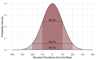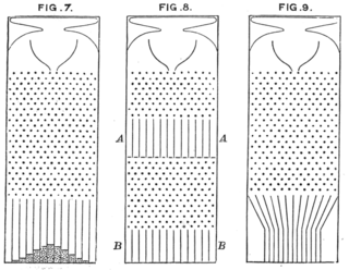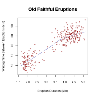
A descriptive statistic is a summary statistic that quantitatively describes or summarizes features from a collection of information, while descriptive statistics is the process of using and analysing those statistics. Descriptive statistics is distinguished from inferential statistics by its aim to summarize a sample, rather than use the data to learn about the population that the sample of data is thought to represent. This generally means that descriptive statistics, unlike inferential statistics, is not developed on the basis of probability theory, and are frequently nonparametric statistics. Even when a data analysis draws its main conclusions using inferential statistics, descriptive statistics are generally also presented. For example, in papers reporting on human subjects, typically a table is included giving the overall sample size, sample sizes in important subgroups, and demographic or clinical characteristics such as the average age, the proportion of subjects of each sex, the proportion of subjects with related co-morbidities, etc.
Multivariate statistics is a subdivision of statistics encompassing the simultaneous observation and analysis of more than one outcome variable, i.e., multivariate random variables. Multivariate statistics concerns understanding the different aims and background of each of the different forms of multivariate analysis, and how they relate to each other. The practical application of multivariate statistics to a particular problem may involve several types of univariate and multivariate analyses in order to understand the relationships between variables and their relevance to the problem being studied.

Statistics is the discipline that concerns the collection, organization, analysis, interpretation, and presentation of data. In applying statistics to a scientific, industrial, or social problem, it is conventional to begin with a statistical population or a statistical model to be studied. Populations can be diverse groups of people or objects such as "all people living in a country" or "every atom composing a crystal". Statistics deals with every aspect of data, including the planning of data collection in terms of the design of surveys and experiments.

In statistics, correlation or dependence is any statistical relationship, whether causal or not, between two random variables or bivariate data. Although in the broadest sense, "correlation" may indicate any type of association, in statistics it usually refers to the degree to which a pair of variables are linearly related. Familiar examples of dependent phenomena include the correlation between the height of parents and their offspring, and the correlation between the price of a good and the quantity the consumers are willing to purchase, as it is depicted in the so-called demand curve.

In statistics, regression toward the mean is the phenomenon where if one sample of a random variable is extreme, the next sampling of the same random variable is likely to be closer to its mean. Furthermore, when many random variables are sampled and the most extreme results are intentionally picked out, it refers to the fact that a second sampling of these picked-out variables will result in "less extreme" results, closer to the initial mean of all of the variables.

In statistics, the Pearson correlation coefficient (PCC) is a correlation coefficient that measures linear correlation between two sets of data. It is the ratio between the covariance of two variables and the product of their standard deviations; thus, it is essentially a normalized measurement of the covariance, such that the result always has a value between −1 and 1. As with covariance itself, the measure can only reflect a linear correlation of variables, and ignores many other types of relationships or correlations. As a simple example, one would expect the age and height of a sample of teenagers from a high school to have a Pearson correlation coefficient significantly greater than 0, but less than 1.

A scatter plot, also called a scatterplot, scatter graph, scatter chart, scattergram, or scatter diagram, is a type of plot or mathematical diagram using Cartesian coordinates to display values for typically two variables for a set of data. If the points are coded (color/shape/size), one additional variable can be displayed. The data are displayed as a collection of points, each having the value of one variable determining the position on the horizontal axis and the value of the other variable determining the position on the vertical axis.

A variable is considered dependent if it depends on an independent variable. Dependent variables are studied under the supposition or demand that they depend, by some law or rule, on the values of other variables. Independent variables, in turn, are not seen as depending on any other variable in the scope of the experiment in question. In this sense, some common independent variables are time, space, density, mass, fluid flow rate, and previous values of some observed value of interest to predict future values.
In statistics, a categorical variable is a variable that can take on one of a limited, and usually fixed, number of possible values, assigning each individual or other unit of observation to a particular group or nominal category on the basis of some qualitative property. In computer science and some branches of mathematics, categorical variables are referred to as enumerations or enumerated types. Commonly, each of the possible values of a categorical variable is referred to as a level. The probability distribution associated with a random categorical variable is called a categorical distribution.
In statistics, a contingency table is a type of table in a matrix format that displays the multivariate frequency distribution of the variables. They are heavily used in survey research, business intelligence, engineering, and scientific research. They provide a basic picture of the interrelation between two variables and can help find interactions between them. The term contingency table was first used by Karl Pearson in "On the Theory of Contingency and Its Relation to Association and Normal Correlation", part of the Drapers' Company Research Memoirs Biometric Series I published in 1904.
This glossary of statistics and probability is a list of definitions of terms and concepts used in the mathematical sciences of statistics and probability, their sub-disciplines, and related fields. For additional related terms, see Glossary of mathematics and Glossary of experimental design.

Local regression or local polynomial regression, also known as moving regression, is a generalization of the moving average and polynomial regression. Its most common methods, initially developed for scatterplot smoothing, are LOESS and LOWESS, both pronounced LOH-ess. They are two strongly related non-parametric regression methods that combine multiple regression models in a k-nearest-neighbor-based meta-model. In some fields, LOESS is known and commonly referred to as Savitzky–Golay filter.

Anscombe's quartet comprises four datasets that have nearly identical simple descriptive statistics, yet have very different distributions and appear very different when graphed. Each dataset consists of eleven (x, y) points. They were constructed in 1973 by the statistician Francis Anscombe to demonstrate both the importance of graphing data when analyzing it, and the effect of outliers and other influential observations on statistical properties. He described the article as being intended to counter the impression among statisticians that "numerical calculations are exact, but graphs are rough".
In statistics, regression validation is the process of deciding whether the numerical results quantifying hypothesized relationships between variables, obtained from regression analysis, are acceptable as descriptions of the data. The validation process can involve analyzing the goodness of fit of the regression, analyzing whether the regression residuals are random, and checking whether the model's predictive performance deteriorates substantially when applied to data that were not used in model estimation.

A plot is a graphical technique for representing a data set, usually as a graph showing the relationship between two or more variables. The plot can be drawn by hand or by a computer. In the past, sometimes mechanical or electronic plotters were used. Graphs are a visual representation of the relationship between variables, which are very useful for humans who can then quickly derive an understanding which may not have come from lists of values. Given a scale or ruler, graphs can also be used to read off the value of an unknown variable plotted as a function of a known one, but this can also be done with data presented in tabular form. Graphs of functions are used in mathematics, sciences, engineering, technology, finance, and other areas.
The following outline is provided as an overview of and topical guide to regression analysis:
In statistics, several scatterplot smoothing methods are available to fit a function through the points of a scatterplot to best represent the relationship between the variables.
A correlation coefficient is a numerical measure of some type of linear correlation, meaning a statistical relationship between two variables. The variables may be two columns of a given data set of observations, often called a sample, or two components of a multivariate random variable with a known distribution.

Bivariate analysis is one of the simplest forms of quantitative (statistical) analysis. It involves the analysis of two variables, for the purpose of determining the empirical relationship between them.
In statistics, linear regression is a statistical model which estimates the linear relationship between a scalar response and one or more explanatory variables. The case of one explanatory variable is called simple linear regression; for more than one, the process is called multiple linear regression. This term is distinct from multivariate linear regression, where multiple correlated dependent variables are predicted, rather than a single scalar variable. If the explanatory variables are measured with error then errors-in-variables models are required, also known as measurement error models.

