
In mathematical physics and mathematics, the Pauli matrices are a set of three 2 × 2 complex matrices that are traceless, Hermitian, involutory and unitary. Usually indicated by the Greek letter sigma, they are occasionally denoted by tau when used in connection with isospin symmetries.

In astronomy, coordinate systems are used for specifying positions of celestial objects relative to a given reference frame, based on physical reference points available to a situated observer. Coordinate systems in astronomy can specify an object's relative position in three-dimensional space or plot merely by its direction on a celestial sphere, if the object's distance is unknown or trivial.
In mechanics and geometry, the 3D rotation group, often denoted SO(3), is the group of all rotations about the origin of three-dimensional Euclidean space under the operation of composition.
In the mathematical field of differential geometry, a metric tensor is an additional structure on a manifold M that allows defining distances and angles, just as the inner product on a Euclidean space allows defining distances and angles there. More precisely, a metric tensor at a point p of M is a bilinear form defined on the tangent space at p, and a metric field on M consists of a metric tensor at each point p of M that varies smoothly with p.
In mathematics, a Gaussian function, often simply referred to as a Gaussian, is a function of the base form and with parametric extension for arbitrary real constants a, b and non-zero c. It is named after the mathematician Carl Friedrich Gauss. The graph of a Gaussian is a characteristic symmetric "bell curve" shape. The parameter a is the height of the curve's peak, b is the position of the center of the peak, and c controls the width of the "bell".
Linear elasticity is a mathematical model as to how solid objects deform and become internally stressed by prescribed loading conditions. It is a simplification of the more general nonlinear theory of elasticity and a branch of continuum mechanics.
In information geometry, the Fisher information metric is a particular Riemannian metric which can be defined on a smooth statistical manifold, i.e., a smooth manifold whose points are probability measures defined on a common probability space. It can be used to calculate the informational difference between measurements.

In quantum mechanics and quantum field theory, the propagator is a function that specifies the probability amplitude for a particle to travel from one place to another in a given period of time, or to travel with a certain energy and momentum. In Feynman diagrams, which serve to calculate the rate of collisions in quantum field theory, virtual particles contribute their propagator to the rate of the scattering event described by the respective diagram. Propagators may also be viewed as the inverse of the wave operator appropriate to the particle, and are, therefore, often called (causal) Green's functions.
In physics, the Hamilton–Jacobi equation, named after William Rowan Hamilton and Carl Gustav Jacob Jacobi, is an alternative formulation of classical mechanics, equivalent to other formulations such as Newton's laws of motion, Lagrangian mechanics and Hamiltonian mechanics.
In mathematics, a Killing vector field, named after Wilhelm Killing, is a vector field on a Riemannian manifold that preserves the metric. Killing fields are the infinitesimal generators of isometries; that is, flows generated by Killing fields are continuous isometries of the manifold. More simply, the flow generates a symmetry, in the sense that moving each point of an object the same distance in the direction of the Killing vector will not distort distances on the object.
The Kerr–Newman metric describes the spacetime geometry around a mass which is electrically charged and rotating. It is a vacuum solution which generalizes the Kerr metric by additionally taking into account the energy of an electromagnetic field, making it the most general asymptotically flat and stationary solution of the Einstein–Maxwell equations in general relativity. As an electrovacuum solution, it only includes those charges associated with the magnetic field; it does not include any free electric charges.
In probability and statistics, a circular distribution or polar distribution is a probability distribution of a random variable whose values are angles, usually taken to be in the range [0, 2π). A circular distribution is often a continuous probability distribution, and hence has a probability density, but such distributions can also be discrete, in which case they are called circular lattice distributions. Circular distributions can be used even when the variables concerned are not explicitly angles: the main consideration is that there is not usually any real distinction between events occurring at the opposite ends of the range, and the division of the range could notionally be made at any point.
The Schwarzschild solution describes spacetime under the influence of a massive, non-rotating, spherically symmetric object. It is considered by some to be one of the simplest and most useful solutions to the Einstein field equations.
In general relativity, the Gibbons–Hawking–York boundary term is a term that needs to be added to the Einstein–Hilbert action when the underlying spacetime manifold has a boundary.
In the mathematical description of general relativity, the Boyer–Lindquist coordinates are a generalization of the coordinates used for the metric of a Schwarzschild black hole that can be used to express the metric of a Kerr black hole.
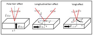
The Voigt effect is a magneto-optical phenomenon which rotates and elliptizes linearly polarised light sent into an optically active medium. The effect is named after the German scientist Woldemar Voigt who discovered it in vapors. Unlike many other magneto-optical effects such as the Kerr or Faraday effect which are linearly proportional to the magnetization, the Voigt effect is proportional to the square of the magnetization and can be seen experimentally at normal incidence. There are also other denominations for this effect, used interchangeably in the modern scientific literature: the Cotton–Mouton effect and magnetic-linear birefringence, with the latter reflecting the physical meaning of the effect.
In the differential geometry of surfaces, a Darboux frame is a natural moving frame constructed on a surface. It is the analog of the Frenet–Serret frame as applied to surface geometry. A Darboux frame exists at any non-umbilic point of a surface embedded in Euclidean space. It is named after French mathematician Jean Gaston Darboux.
In mathematics, vector spherical harmonics (VSH) are an extension of the scalar spherical harmonics for use with vector fields. The components of the VSH are complex-valued functions expressed in the spherical coordinate basis vectors.
The Carter constant is a conserved quantity for motion around black holes in the general relativistic formulation of gravity. Its SI base units are kg2⋅m4⋅s−2. Carter's constant was derived for a spinning, charged black hole by Australian theoretical physicist Brandon Carter in 1968. Carter's constant along with the energy , axial angular momentum , and particle rest mass provide the four conserved quantities necessary to uniquely determine all orbits in the Kerr–Newman spacetime.
Chandrasekhar–Page equations describe the wave function of the spin-1/2 massive particles, that resulted by seeking a separable solution to the Dirac equation in Kerr metric or Kerr–Newman metric. In 1976, Subrahmanyan Chandrasekhar showed that a separable solution can be obtained from the Dirac equation in Kerr metric. Later, Don Page extended this work to Kerr–Newman metric, that is applicable to charged black holes. In his paper, Page notices that N. Toop also derived his results independently, as informed to him by Chandrasekhar.


