Continuous gusts

Last updated

Continuous gusts or stochastic gusts are winds that vary randomly in space and time. Models of continuous gusts are used to represent atmospheric turbulence, especially clear air turbulence and turbulent winds in storms. The Federal Aviation Administration (FAA) and the United States Department of Defense provide requirements for the models of continuous gusts used in design and simulation of aircraft. [1] [2]

Contents

Models of continuous gusts

A variety of models exist for gusts [3] but only two, the Dryden and von Kármán models, are generally used for continuous gusts in flight dynamics applications. [2] [4] Both of these models define gusts in terms of power spectral densities for the linear and angular velocity components parameterized by turbulence length scales and intensities. The velocity components of these continuous gust models can be incorporated into airplane equations of motion as a wind disturbance. [5] While these models of continuous gusts are not white noise, filters can be designed that take a white noise input and output a random process with the Dryden or von Kármán models. [6] [7]

Assumptions of continuous gust models

The models accepted by the FAA and Department of Defense represent continuous gusts as a wind linear and angular velocity field that is a random process and make a number of simplifying assumptions in order to describe them mathematically. In particular, continuous gusts are assumed to be: [8]

These assumptions, while unrealistic, yield acceptable models for flight dynamics applications. [9] The last assumption of a velocity field that does not vary with time is especially unrealistic, since measurements of atmospheric turbulence at one point in space always vary with time. These models rely on the airplane's motion through the gusts to generate temporal variations in wind velocity, making them inappropriate for use as inputs to models of hovering, wind turbines, or other applications that are fixed in space.

The models also make assumptions about how continuous gusts vary with altitude. The Dryden and von Kármán models specified by the Department of Defense define three different altitude ranges: low, 10 ft to 1000 ft AGL; medium/high, 2000 ft AGL and above; and in between. The turbulence intensities, turbulence scale lengths, and turbulence axes depend on the altitude. [10] The Department of Defense also provides models for the gust angular velocity but gives criteria based on airplane stability derivatives for when they can be omitted. [11]

Dryden model

The Dryden model is one of the most commonly used models of continuous gusts. It was first published in 1952. [12] The power spectral density of the longitudinal linear velocity component is

where ug is the gusts' longitudinal linear velocity component, σu is the turbulence intensity, Lu is the turbulence scale length, and Ω is a spatial frequency. [2]

The Dryden model has rational power spectral densities for each velocity component. This means that an exact filter can be formed that takes white noise as an input and outputs a random process with the Dryden model's power spectral densities. [6]

von Kármán model

The von Kármán model is the preferred model of continuous gusts for the Department of Defense and the FAA. [1] [2] The model first appeared in a 1957 NACA report [13] based on earlier work by Theodore von Kármán. [14] [15] [16] In this model, the power spectral density of the longitudinal linear velocity component is

where ug is the longitudinal linear velocity component, σu is the turbulence intensity, Lu is the turbulence scale length, and Ω is a spatial frequency. [2]

The von Kármán model has irrational power spectral densities. So, a filter with a white noise input that outputs a random process with the von Kármán model's power spectral densities can only be approximated. [7]

Altitude dependence

Both the Dryden and von Kármán models are parameterized by a length scale and turbulence intensity. The combination of these two parameters determine the shape of the power spectral densities and therefore the quality of the models' fit to spectra of observed turbulence. Many combinations of length scale and turbulence intensity give realistic power spectral densities in the desired frequency ranges. [4] The Department of Defense specifications include choices for both parameters, including their dependence on altitude, which are summarized below. [10]

Low altitude

Low altitude is defined as altitudes between 10 ft AGL and 1000 ft AGL.

Length scales

At low altitude, the scale lengths are functions of altitude,

where h is the altitude AGL. At 1000 ft AGL, Lu = 2Lv = 2Lw = 1000 ft.

Turbulence intensities

At low altitude, the turbulence intensities are parameterized by W20, the wind speed at 20 ft.

Turbulence severity
Light15 kts
Moderate30 kts
Severe45 kts

At 1000 ft AGL,

Medium/high altitude

Medium/high altitude is defined as 2000 ft AGL and above.

Turbulence intensity vs. altitude for medium/high altitudes. Turbulence Severity and Exceedance Probability Chart MIL-HDBK-1797.png
Turbulence intensity vs. altitude for medium/high altitudes.

Length scales

For the Dryden model,

For the von Kármán model,

Turbulence intensities

At high altitude,

They are parameterized by the probability of exceedance or the turbulence severity. A plot of turbulence intensity versus altitude showing lines of constant probability of exceedance and ranges corresponding to different turbulence severities is provided in the military specifications. [17]

Between low and medium/high altitude

From 1000 ft AGL to 2000 ft AGL, both the length scale and turbulence intensity are determined by linear interpolation between the low altitude value at 1000 ft and the medium/high altitude value at 2000 ft. [6] [7]

Turbulence axes

Above 1750 ft, the axes of the turbulence coincide with the wind frame axes. Below 1750 ft, the vertical turbulence axis is aligned with the Earth frame z-axis, the longitudinal turbulence axis is aligned with the projection of the mean wind vector onto the Earth frame's horizontal plane, and the lateral turbulence axis is determined by the right hand rule. [18]

See also

Notes

  1. 1 2 14 CFR Part 25: Appendix G (2011). "Airworthiness Standards: Transport Category Airplanes". U.S. Code of Federal Regulations. Government Printing Office.
  2. 1 2 3 4 5 MIL-STD-1797A 1990, p. 678.
  3. MIL-STD-1797A 1990, pp. 695–697.
  4. 1 2 Hoblit 1988, Chap. 4.
  5. Etkin 2005, pp. 543–562.
  6. 1 2 3 "Dryden Wind Turbulence Model (Continuous)". MATLAB Reference Pages. The MathWorks, Inc. 2010. Retrieved May 24, 2013.
  7. 1 2 3 "Von Karman Wind Turbulence Model (Continuous)". MATLAB Reference Pages. The MathWorks, Inc. 2010. Retrieved May 24, 2013.
  8. Etkin 2005, pp. 531–543.
  9. Hoblit 1988, Chap. 12.
  10. 1 2 MIL-STD-1797A 1990, pp. 673, 678–685, 702.
  11. MIL-STD-1797A 1990, p. 680.
  12. Liepmann, H. W. (1952). "On the Application of Statistical Concepts to the Buffeting Problem". Journal of the Aeronautical Sciences. 19 (12): 793–800. doi:10.2514/8.2491.
  13. Diedrich, Franklin W.; Joseph A. Drischler (1957). Effect of Spanwise Variations in Gust Intensity on the Lift Due to Atmospheric Turbulence (Report). pp. NACA TN 3920.
  14. de Kármán, Theodore; Leslie Howarth (1938). "On the Statistical Theory of Isotropic Turbulence". Proceedings of the Royal Society of London. Series A, Mathematical and Physical Sciences. 164 (917): 192–215. Bibcode:1938RSPSA.164..192D. doi:10.1098/rspa.1938.0013.
  15. von Kármán, Theodore (1948). "Progress in the Statistical Theory of Turbulence". Proceedings of the National Academy of Sciences. 34 (11): 530–539. Bibcode:1948PNAS...34..530V. doi: 10.1073/pnas.34.11.530 . PMC   1079162 . PMID   16588830.
  16. von Kármán, T.; Lin, C. C. (1951). "On the Statistical Theory of Isotropic Turbulence". In von Mises, Richard; von Kármán, Theodore (eds.). Advances in Applied Mechanics. Academic Press, Inc. pp. 1–19. ISBN   9780080563800.
  17. MIL-STD-1797A 1990, p. 673.
  18. MIL-STD-1797A 1990, p. 702.

Related Research Articles

<span class="mw-page-title-main">Brownian motion</span> Random motion of particles suspended in a fluid

Brownian motion is the random motion of particles suspended in a medium.

In physics, the cross section is a measure of the probability that a specific process will take place when some kind of radiant excitation intersects a localized phenomenon. For example, the Rutherford cross-section is a measure of probability that an alpha particle will be deflected by a given angle during an interaction with an atomic nucleus. Cross section is typically denoted σ (sigma) and is expressed in units of area, more specifically in barns. In a way, it can be thought of as the size of the object that the excitation must hit in order for the process to occur, but more exactly, it is a parameter of a stochastic process.

<span class="mw-page-title-main">Active laser medium</span> Source of optical gain in a laser

The active laser medium is the source of optical gain within a laser. The gain results from the stimulated emission of photons through electronic or molecular transitions to a lower energy state from a higher energy state previously populated by a pump source.

<span class="mw-page-title-main">Stefan–Boltzmann law</span> Physical law on the emissive power of black body

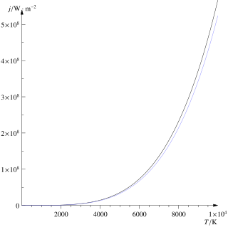
The Stefan–Boltzmann law, also known as Stefan's law, describes the intensity of the thermal radiation emitted by matter in terms of that matter's temperature. It is named for Josef Stefan, who empirically derived the relationship, and Ludwig Boltzmann who derived the law theoretically.

<span class="mw-page-title-main">Rayleigh distribution</span> Probability distribution

In probability theory and statistics, the Rayleigh distribution is a continuous probability distribution for nonnegative-valued random variables. Up to rescaling, it coincides with the chi distribution with two degrees of freedom. The distribution is named after Lord Rayleigh.

The primitive equations are a set of nonlinear partial differential equations that are used to approximate global atmospheric flow and are used in most atmospheric models. They consist of three main sets of balance equations:

  1. A continuity equation: Representing the conservation of mass.
  2. Conservation of momentum: Consisting of a form of the Navier–Stokes equations that describe hydrodynamical flow on the surface of a sphere under the assumption that vertical motion is much smaller than horizontal motion (hydrostasis) and that the fluid layer depth is small compared to the radius of the sphere
  3. A thermal energy equation: Relating the overall temperature of the system to heat sources and sinks
<span class="mw-page-title-main">Lattice Boltzmann methods</span> Class of computational fluid dynamics methods

The lattice Boltzmann methods (LBM), originated from the lattice gas automata (LGA) method (Hardy-Pomeau-Pazzis and Frisch-Hasslacher-Pomeau models), is a class of computational fluid dynamics (CFD) methods for fluid simulation. Instead of solving the Navier–Stokes equations directly, a fluid density on a lattice is simulated with streaming and collision (relaxation) processes. The method is versatile as the model fluid can straightforwardly be made to mimic common fluid behaviour like vapour/liquid coexistence, and so fluid systems such as liquid droplets can be simulated. Also, fluids in complex environments such as porous media can be straightforwardly simulated, whereas with complex boundaries other CFD methods can be hard to work with.

In fluid dynamics, turbulence kinetic energy (TKE) is the mean kinetic energy per unit mass associated with eddies in turbulent flow. Physically, the turbulence kinetic energy is characterised by measured root-mean-square (RMS) velocity fluctuations. In the Reynolds-averaged Navier Stokes equations, the turbulence kinetic energy can be calculated based on the closure method, i.e. a turbulence model.

In physics, the Spalart–Allmaras model is a one-equation model that solves a modelled transport equation for the kinematic eddy turbulent viscosity. The Spalart–Allmaras model was designed specifically for aerospace applications involving wall-bounded flows and has been shown to give good results for boundary layers subjected to adverse pressure gradients. It is also gaining popularity in turbomachinery applications.

In fluid dynamics, the von Kármán constant, named for Theodore von Kármán, is a dimensionless constant involved in the logarithmic law describing the distribution of the longitudinal velocity in the wall-normal direction of a turbulent fluid flow near a boundary with a no-slip condition. The equation for such boundary layer flow profiles is:

Atmospheric tides are global-scale periodic oscillations of the atmosphere. In many ways they are analogous to ocean tides. Atmospheric tides can be excited by:

The intent of this article is to highlight the important points of the derivation of the Navier–Stokes equations as well as its application and formulation for different families of fluids.

The McCumber relation is a relationship between the effective cross-sections of absorption and emission of light in the physics of solid-state lasers. It is named after Dean McCumber, who proposed the relationship in 1964.

The Föppl–von Kármán equations, named after August Föppl and Theodore von Kármán, are a set of nonlinear partial differential equations describing the large deflections of thin flat plates. With applications ranging from the design of submarine hulls to the mechanical properties of cell wall, the equations are notoriously difficult to solve, and take the following form:

The Dryden wind turbulence model, also known as Dryden gusts, is a mathematical model of continuous gusts accepted for use by the United States Department of Defense in certain aircraft design and simulation applications. The Dryden model treats the linear and angular velocity components of continuous gusts as spatially varying stochastic processes and specifies each component's power spectral density. The Dryden wind turbulence model is characterized by rational power spectral densities, so exact filters can be designed that take white noise inputs and output stochastic processes with the Dryden gusts' power spectral densities.

The von Kármán wind turbulence model is a mathematical model of continuous gusts. It matches observed continuous gusts better than that Dryden Wind Turbulence Model and is the preferred model of the United States Department of Defense in most aircraft design and simulation applications. The von Kármán model treats the linear and angular velocity components of continuous gusts as spatially varying stochastic processes and specifies each component's power spectral density. The von Kármán wind turbulence model is characterized by irrational power spectral densities, so filters can be designed that take white noise inputs and output stochastic processes with the approximated von Kármán gusts' power spectral densities.

The Sandia method is a method for generating a turbulent wind profile that can be used in aero-elastic software to evaluate the fatigue imparted on a turbine in a turbulent environment. That is, it generates time series of wind speeds at a set of points on a surface, say the plane of the rotor of a wind turbine. Analysis is performed initially in the frequency domain, where turbulence can be described quantitatively with more ease than the time domain. Then, the time series are obtained by inverse fast Fourier transforms.

Reynolds stress equation model (RSM), also referred to as second moment closures are the most complete classical turbulence model. In these models, the eddy-viscosity hypothesis is avoided and the individual components of the Reynolds stress tensor are directly computed. These models use the exact Reynolds stress transport equation for their formulation. They account for the directional effects of the Reynolds stresses and the complex interactions in turbulent flows. Reynolds stress models offer significantly better accuracy than eddy-viscosity based turbulence models, while being computationally cheaper than Direct Numerical Simulations (DNS) and Large Eddy Simulations.

In computational fluid dynamics, the k–omega (k–ω) turbulence model is a common two-equation turbulence model, that is used as an approximation for the Reynolds-averaged Navier–Stokes equations (RANS equations). The model attempts to predict turbulence by two partial differential equations for two variables, k and ω, with the first variable being the turbulence kinetic energy (k) while the second (ω) is the specific rate of dissipation (of the turbulence kinetic energy k into internal thermal energy).

Menter's Shear Stress Transport turbulence model, or SST, is a widely used and robust two-equation eddy-viscosity turbulence model used in Computational Fluid Dynamics. The model combines the k-omega turbulence model and K-epsilon turbulence model such that the k-omega is used in the inner region of the boundary layer and switches to the k-epsilon in the free shear flow.

References