Source separation, blind signal separation (BSS) or blind source separation, is the separation of a set of source signals from a set of mixed signals, without the aid of information about the source signals or the mixing process. It is most commonly applied in digital signal processing and involves the analysis of mixtures of signals; the objective is to recover the original component signals from a mixture signal. The classical example of a source separation problem is the cocktail party problem, where a number of people are talking simultaneously in a room, and a listener is trying to follow one of the discussions. The human brain can handle this sort of auditory source separation problem, but it is a difficult problem in digital signal processing.
In statistics, maximum likelihood estimation (MLE) is a method of estimating the parameters of an assumed probability distribution, given some observed data. This is achieved by maximizing a likelihood function so that, under the assumed statistical model, the observed data is most probable. The point in the parameter space that maximizes the likelihood function is called the maximum likelihood estimate. The logic of maximum likelihood is both intuitive and flexible, and as such the method has become a dominant means of statistical inference.
In statistics, the Gauss–Markov theorem states that the ordinary least squares (OLS) estimator has the lowest sampling variance within the class of linear unbiased estimators, if the errors in the linear regression model are uncorrelated, have equal variances and expectation value of zero. The errors do not need to be normal for the theorem to apply, nor do they need to be independent and identically distributed.

In statistics, the logistic model is a statistical model that models the log-odds of an event as a linear combination of one or more independent variables. In regression analysis, logistic regression is estimating the parameters of a logistic model. Formally, in binary logistic regression there is a single binary dependent variable, coded by an indicator variable, where the two values are labeled "0" and "1", while the independent variables can each be a binary variable or a continuous variable. The corresponding probability of the value labeled "1" can vary between 0 and 1, hence the labeling; the function that converts log-odds to probability is the logistic function, hence the name. The unit of measurement for the log-odds scale is called a logit, from logistic unit, hence the alternative names. See § Background and § Definition for formal mathematics, and § Example for a worked example.
In signal processing, independent component analysis (ICA) is a computational method for separating a multivariate signal into additive subcomponents. This is done by assuming that at most one subcomponent is Gaussian and that the subcomponents are statistically independent from each other. ICA is a special case of blind source separation. A common example application is the "cocktail party problem" of listening in on one person's speech in a noisy room.
In statistics, a studentized residual is the dimensionless ratio resulting from the division of a residual by an estimate of its standard deviation, both expressed in the same units. It is a form of a Student's t-statistic, with the estimate of error varying between points.

In statistical modeling, regression analysis is a set of statistical processes for estimating the relationships between a dependent variable and one or more independent variables. The most common form of regression analysis is linear regression, in which one finds the line that most closely fits the data according to a specific mathematical criterion. For example, the method of ordinary least squares computes the unique line that minimizes the sum of squared differences between the true data and that line. For specific mathematical reasons, this allows the researcher to estimate the conditional expectation of the dependent variable when the independent variables take on a given set of values. Less common forms of regression use slightly different procedures to estimate alternative location parameters or estimate the conditional expectation across a broader collection of non-linear models.
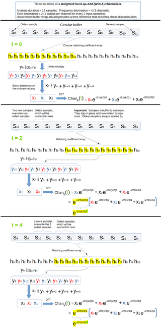
In signal processing, a filter bank is an array of bandpass filters that separates the input signal into multiple components, each one carrying a single frequency sub-band of the original signal. One application of a filter bank is a graphic equalizer, which can attenuate the components differently and recombine them into a modified version of the original signal. The process of decomposition performed by the filter bank is called analysis ; the output of analysis is referred to as a subband signal with as many subbands as there are filters in the filter bank. The reconstruction process is called synthesis, meaning reconstitution of a complete signal resulting from the filtering process.
In statistics, the residual sum of squares (RSS), also known as the sum of squared residuals (SSR) or the sum of squared estimate of errors (SSE), is the sum of the squares of residuals. It is a measure of the discrepancy between the data and an estimation model, such as a linear regression. A small RSS indicates a tight fit of the model to the data. It is used as an optimality criterion in parameter selection and model selection.

In statistics, simple linear regression (SLR) is a linear regression model with a single explanatory variable. That is, it concerns two-dimensional sample points with one independent variable and one dependent variable and finds a linear function that, as accurately as possible, predicts the dependent variable values as a function of the independent variable. The adjective simple refers to the fact that the outcome variable is related to a single predictor.
The topic of heteroskedasticity-consistent (HC) standard errors arises in statistics and econometrics in the context of linear regression and time series analysis. These are also known as heteroskedasticity-robust standard errors, Eicker–Huber–White standard errors, to recognize the contributions of Friedhelm Eicker, Peter J. Huber, and Halbert White.
In statistics, principal component regression (PCR) is a regression analysis technique that is based on principal component analysis (PCA). More specifically, PCR is used for estimating the unknown regression coefficients in a standard linear regression model.
In statistics, a sum of squares due to lack of fit, or more tersely a lack-of-fit sum of squares, is one of the components of a partition of the sum of squares of residuals in an analysis of variance, used in the numerator in an F-test of the null hypothesis that says that a proposed model fits well. The other component is the pure-error sum of squares.
In statistics and in particular in regression analysis, leverage is a measure of how far away the independent variable values of an observation are from those of the other observations. High-leverage points, if any, are outliers with respect to the independent variables. That is, high-leverage points have no neighboring points in space, where is the number of independent variables in a regression model. This makes the fitted model likely to pass close to a high leverage observation. Hence high-leverage points have the potential to cause large changes in the parameter estimates when they are deleted i.e., to be influential points. Although an influential point will typically have high leverage, a high leverage point is not necessarily an influential point. The leverage is typically defined as the diagonal elements of the hat matrix.
Uniform convergence in probability is a form of convergence in probability in statistical asymptotic theory and probability theory. It means that, under certain conditions, the empirical frequencies of all events in a certain event-family converge to their theoretical probabilities. Uniform convergence in probability has applications to statistics as well as machine learning as part of statistical learning theory.
The purpose of this page is to provide supplementary materials for the ordinary least squares article, reducing the load of the main article with mathematics and improving its accessibility, while at the same time retaining the completeness of exposition.

Symmetries in quantum mechanics describe features of spacetime and particles which are unchanged under some transformation, in the context of quantum mechanics, relativistic quantum mechanics and quantum field theory, and with applications in the mathematical formulation of the standard model and condensed matter physics. In general, symmetry in physics, invariance, and conservation laws, are fundamentally important constraints for formulating physical theories and models. In practice, they are powerful methods for solving problems and predicting what can happen. While conservation laws do not always give the answer to the problem directly, they form the correct constraints and the first steps to solving a multitude of problems. In application, understanding symmetries can also provide insights on the eigenstates that can be expected. For example, the existence of degenerate states can be inferred by the presence of non commuting symmetry operators or that the non degenerate states are also eigenvectors of symmetry operators.
In pure and applied mathematics, quantum mechanics and computer graphics, a tensor operator generalizes the notion of operators which are scalars and vectors. A special class of these are spherical tensor operators which apply the notion of the spherical basis and spherical harmonics. The spherical basis closely relates to the description of angular momentum in quantum mechanics and spherical harmonic functions. The coordinate-free generalization of a tensor operator is known as a representation operator.
IQ imbalance is a performance-limiting issue in the design of a class of radio receivers known as direct conversion receivers. These translate the received radio frequency signal directly from the carrier frequency to baseband using a single mixing stage.
In mathematics, the injective tensor product of two topological vector spaces (TVSs) was introduced by Alexander Grothendieck and was used by him to define nuclear spaces. An injective tensor product is in general not necessarily complete, so its completion is called the completed injective tensor products. Injective tensor products have applications outside of nuclear spaces. In particular, as described below, up to TVS-isomorphism, many TVSs that are defined for real or complex valued functions, for instance, the Schwartz space or the space of continuously differentiable functions, can be immediately extended to functions valued in a Hausdorff locally convex TVS without any need to extend definitions from real/complex-valued functions to -valued functions.


