Elliptic surface

In mathematics, an elliptic surface is a surface that has an elliptic fibration, in other words a proper morphism with connected fibers to an algebraic curve such that almost all fibers are smooth curves of genus 1. (Over an algebraically closed field such as the complex numbers, these fibers are elliptic curves, perhaps without a chosen origin.) This is equivalent to the generic fiber being a smooth curve of genus one. This follows from proper base change.

The surface and the base curve are assumed to be non-singular (complex manifolds or regular schemes, depending on the context). The fibers that are not elliptic curves are called the singular fibers and were classified by Kunihiko Kodaira. Both elliptic and singular fibers are important in string theory, especially in F-theory.

Elliptic surfaces form a large class of surfaces that contains many of the interesting examples of surfaces, and are relatively well understood in the theories of complex manifolds and smooth 4-manifolds. They are similar to (have analogies with, that is), elliptic curves over number fields.

Examples

• The product of any elliptic curve with any curve is an elliptic surface (with no singular fibers).
• All surfaces of Kodaira dimension 1 are elliptic surfaces.
• Every complex Enriques surface is elliptic, and has an elliptic fibration over the projective line.
• Kodaira surfaces
• Dolgachev surfaces
• Shioda modular surfaces

Kodaira's table of singular fibers

Most of the fibers of an elliptic fibration are (non-singular) elliptic curves. The remaining fibers are called singular fibers: there are a finite number of them, and each one consists of a union of rational curves, possibly with singularities or non-zero multiplicities (so the fibers may be non-reduced schemes). Kodaira and Néron independently classified the possible fibers, and Tate's algorithm can be used to find the type of the fibers of an elliptic curve over a number field.

The following table lists the possible fibers of a minimal elliptic fibration. ("Minimal" means roughly one that cannot be factored through a "smaller" one; precisely, the singular fibers should contain no smooth rational curves with self-intersection number −1.) It gives:

• Kodaira's symbol for the fiber,
• André Néron's symbol for the fiber,
• The number of irreducible components of the fiber (all rational except for type I₀)
• The intersection matrix of the components. This is either a 1×1 zero matrix, or an affine Cartan matrix, whose Dynkin diagram is given.
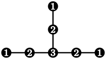
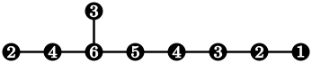
• The multiplicities of each fiber are indicated in the Dynkin diagram.

Kodaira	Néron	Components	Intersection matrix	Dynkin diagram	Fiber
I0	A	1 (elliptic)	0
I1	B1	1 (with double point)	0
I2	B2	2 (2 distinct intersection points)	affine A1
Iv (v≥2)	Bv	v (v distinct intersection points)	affine Av-1
mIv (v≥0, m≥2)		Iv with multiplicity m
II	C1	1 (with cusp)	0
III	C2	2 (meet at one point of order 2)	affine A1
IV	C3	3 (all meet in 1 point)	affine A2
I0*	C4	5	affine D4
Iv* (v≥1)	C5,v	5+v	affine D4+v
IV*	C6	7	affine E6
III*	C7	8	affine E7
II*	C8	9	affine E8

This table can be found as follows. Geometric arguments show that the intersection matrix of the components of the fiber must be negative semidefinite, connected, symmetric, and have no diagonal entries equal to −1 (by minimality). Such a matrix must be 0 or a multiple of the Cartan matrix of an affine Dynkin diagram of type ADE.

The intersection matrix determines the fiber type with three exceptions:

• If the intersection matrix is 0 the fiber can be either an elliptic curve (type I₀), or have a double point (type I₁), or a cusp (type II).
• If the intersection matrix is affine A₁, there are 2 components with intersection multiplicity 2. They can meet either in 2 points with order 1 (type I₂), or at one point with order 2 (type III).
• If the intersection matrix is affine A₂, there are 3 components each meeting the other two. They can meet either in pairs at 3 distinct points (type I₃), or all meet at the same point (type IV).

Monodromy

The monodromy around each singular fiber is a well-defined conjugacy class in the group SL(2,Z) of 2 × 2 integer matrices with determinant 1. The monodromy describes the way the first homology group of a smooth fiber (which is isomorphic to Z²) changes as we go around a singular fiber. Representatives for these conjugacy classes associated to singular fibers are given by: ^[1]

Fiber	Intersection matrix	Monodromy	j-invariant	Group structure on smooth locus
Iν	affine Aν-1	${\displaystyle {\begin{pmatrix}1&\nu \\0&1\end{pmatrix}}}$	${\displaystyle \infty }$	${\displaystyle \mathbf {Z} /\nu \times \mathbf {C} ^{*}}$
II	0	${\displaystyle {\begin{pmatrix}1&1\\-1&0\end{pmatrix}}}$	0	${\displaystyle \mathbf {C} }$
III	affine A1	${\displaystyle {\begin{pmatrix}0&1\\-1&0\end{pmatrix}}}$	1728	${\displaystyle \mathbf {Z} /2\times \mathbf {C} }$
IV	affine A2	${\displaystyle {\begin{pmatrix}0&1\\-1&-1\end{pmatrix}}}$	0	${\displaystyle \mathbf {Z} /3\times \mathbf {C} }$
I0*	affine D4	${\displaystyle {\begin{pmatrix}-1&0\\0&-1\end{pmatrix}}}$	in ${\displaystyle \mathbf {C} }$	${\displaystyle (\mathbf {Z} /2)^{2}\times \mathbf {C} }$
Iν* (ν≥1)	affine D4+ν	${\displaystyle {\begin{pmatrix}-1&-\nu \\0&-1\end{pmatrix}}}$	${\displaystyle \infty }$	${\displaystyle (\mathbf {Z} /2)^{2}\times \mathbf {C} }$ if ν is even, ${\displaystyle \mathbf {Z} /4\times \mathbf {C} }$ if ν is odd
IV*	affine E6	${\displaystyle {\begin{pmatrix}-1&-1\\1&0\end{pmatrix}}}$	0	${\displaystyle \mathbf {Z} /3\times \mathbf {C} }$
III*	affine E7	${\displaystyle {\begin{pmatrix}0&-1\\1&0\end{pmatrix}}}$	1728	${\displaystyle \mathbf {Z} /2\times \mathbf {C} }$
II*	affine E8	${\displaystyle {\begin{pmatrix}0&-1\\1&1\end{pmatrix}}}$	0	${\displaystyle \mathbf {C} }$

For singular fibers of type II, III, IV, I₀^*, IV^*, III^*, or II^*, the monodromy has finite order in SL(2,Z). This reflects the fact that an elliptic fibration has potential good reduction at such a fiber. That is, after a ramified finite covering of the base curve, the singular fiber can be replaced by a smooth elliptic curve. Which smooth curve appears is described by the j-invariant in the table. Over the complex numbers, the curve with j-invariant 0 is the unique elliptic curve with automorphism group of order 6, and the curve with j-invariant 1728 is the unique elliptic curve with automorphism group of order 4. (All other elliptic curves have automorphism group of order 2.)

For an elliptic fibration with a section, called a Jacobian elliptic fibration, the smooth locus of each fiber has a group structure. For singular fibers, this group structure on the smooth locus is described in the table, assuming for convenience that the base field is the complex numbers. (For a singular fiber with intersection matrix given by an affine Dynkin diagram ${\displaystyle {\tilde {\Gamma }}}$, the group of components of the smooth locus is isomorphic to the center of the simply connected simple Lie group with Dynkin diagram ${\displaystyle \Gamma }$, as listed here.) Knowing the group structure of the singular fibers is useful for computing the Mordell-Weil group of an elliptic fibration (the group of sections), in particular its torsion subgroup.

Canonical bundle formula

To understand how elliptic surfaces fit into the classification of surfaces, it is important to compute the canonical bundle of a minimal elliptic surface f: X → S. Over the complex numbers, Kodaira proved the following canonical bundle formula: ^[2]

${\displaystyle K_{X}=f^{*}(L)\otimes O_{S}{\big (}\sum _{i}(m_{i}-1)D_{i}{\big )}.}$

Here the multiple fibers of f (if any) are written as ${\displaystyle f^{*}(p_{i})=m_{i}D_{i}}$, for an integer m_i at least 2 and a divisor D_i whose coefficients have greatest common divisor equal to 1, and L is some line bundle on the smooth curve S. If S is projective (or equivalently, compact), then the degree of L is determined by the holomorphic Euler characteristics of X and S: deg(L) = χ(X,O_X) − 2χ(S,O_S). The canonical bundle formula implies that K_X is Q-linearly equivalent to the pullback of some Q-divisor on S; it is essential here that the elliptic surface X → S is minimal.

Building on work of Kenji Ueno, Takao Fujita (1986) gave a useful variant of the canonical bundle formula, showing how K_X depends on the variation of the smooth fibers. ^[3] Namely, there is a Q-linear equivalence

${\displaystyle K_{X}\sim _{\bf {Q}}f^{*}(K_{S}+B_{S}+M_{S}),}$

where the discriminant divisorB_S is an explicit effective Q-divisor on S associated to the singular fibers of f, and the moduli divisorM_S is ${\displaystyle (1/12)j^{*}O(1)}$, where j: S → P¹ is the function giving the j-invariant of the smooth fibers. (Thus M_S is a Q-linear equivalence class of Q-divisors, using the identification between the divisor class group Cl(S) and the Picard group Pic(S).) In particular, for S projective, the moduli divisor M_S has nonnegative degree, and it has degree zero if and only if the elliptic surface is isotrivial, meaning that all the smooth fibers are isomorphic.

The discriminant divisor in Fujita's formula is defined by

${\displaystyle B_{S}=\sum _{p\in S}(1-c(p))[p]}$,

where c(p) is the log canonical threshold${\displaystyle {\text{lct}}(X,f^{*}(p))}$. This is an explicit rational number between 0 and 1, depending on the type of singular fiber. Explicitly, the lct is 1 for a smooth fiber or type ${\displaystyle I_{\nu }}$, and it is 1/m for a multiple fiber ${\displaystyle {}_{m}I_{\nu }}$, 1/2 for ${\displaystyle I_{\nu }^{*}}$, 5/6 for II, 3/4 for III, 2/3 for IV, 1/3 for IV*, 1/4 for III*, and 1/6 for II*.

The canonical bundle formula (in Fujita's form) has been generalized by Yujiro Kawamata and others to families of Calabi–Yau varieties of any dimension. ^[4]

Logarithmic transformations

"Logarithmic transformation" redirects here. Not to be confused with Logarithmic data transformation.

A logarithmic transformation (of order m with center p) of an elliptic surface or fibration turns a fiber of multiplicity 1 over a point p of the base space into a fiber of multiplicity m. It can be reversed, so fibers of high multiplicity can all be turned into fibers of multiplicity 1, and this can be used to eliminate all multiple fibers.

Logarithmic transformations can be quite violent: they can change the Kodaira dimension, and can turn algebraic surfaces into non-algebraic surfaces.

Example: Let L be the lattice Z+iZ of C, and let E be the elliptic curve C/L. Then the projection map from E×C to C is an elliptic fibration. We will show how to replace the fiber over 0 with a fiber of multiplicity 2.

There is an automorphism of E×C of order 2 that maps (c,s) to (c+1/2, −s). We let X be the quotient of E×C by this group action. We make X into a fiber space over C by mapping (c,s) to s². We construct an isomorphism from X minus the fiber over 0 to E×C minus the fiber over 0 by mapping (c,s) to (c-log(s)/2πi,s²). (The two fibers over 0 are non-isomorphic elliptic curves, so the fibration X is certainly not isomorphic to the fibration E×C over all of C.)

Then the fibration X has a fiber of multiplicity 2 over 0, and otherwise looks like E×C. We say that X is obtained by applying a logarithmic transformation of order 2 to E×C with center 0.

See also

• Enriques–Kodaira classification
• Néron minimal model

Notes

1. Barth et al. (2004), section V.10, Tables 5 and 6; Cossec and Dolgachev (1989), Corollary 5.2.3.
2. Barth et al. (2004), Corollary III.12.3.
3. Kollár (2007), section 8.2.
4. Kollár (2007), section 8.5.

References

• Barth, Wolf P.; Hulek, Klaus; Peters, Chris A.M.; Van de Ven, Antonius (2004) [1984], Compact Complex Surfaces, Springer, doi:10.1007/978-3-642-57739-0, ISBN   978-3-540-00832-3, MR   2030225
• Cossec, François; Dolgachev, Igor (1989). Enriques Surfaces. Boston: Birkhäuser. doi:10.1007/978-1-4612-3696-2. ISBN   3-7643-3417-7. MR   0986969.
• Kodaira, Kunihiko (1963). "On compact analytic surfaces. II". Ann. of Math. 77: 563–626. doi:10.2307/1970131. MR   0184257. Zbl   0118.15802.
• Kodaira, Kunihiko (1964). "On the structure of compact complex analytic surfaces. I". Am. J. Math. 86: 751–798. doi:10.2307/2373157. MR   0187255. Zbl   0137.17501.
• Kollár, János (2007), "Kodaira's canonical bundle formula and adjunction", Flips for 3-folds and 4-folds, Oxford University Press, pp. 134–162, doi:10.1093/acprof:oso/9780198570615.003.0008, MR   2359346
• Néron, André (1964). "Modèles minimaux des variétés abéliennes sur les corps locaux et globaux". Publications Mathématiques de l'IHÉS (in French). 21: 5–128. doi:10.1007/BF02684271. MR   0179172. Zbl   0132.41403.