Gipps' model

Gipps' model is a mathematical model for describing car-following behaviour by motorists in the United Kingdom.

The model is named after Peter G. Gipps who developed it in the late-1970s under S.R.C. grants at the Transport Operations Research Group at the University of Newcastle-Upon-Tyne and the Transport Studies Group at the University College London.

Gipps' model is based directly on driver behavior and expectancy for vehicles in a stream of traffic. Limitations on driver and vehicle parameters for safety purposes mimic the traits of vehicles following vehicles in the front of the traffic stream. ^[1] Gipps' model is differentiated by other models in that Gipps uses a timestep within the function equal to ${\displaystyle \tau }$ to reduce the computation required for numerical analysis.

Introduction

The method of modeling individual cars along a continuous space originates with Chandler et al. (1958), Gazis et al. (1961), ^[2] Lee (1966) and Bender and Fenton (1972), ^[3] though many other papers proceeded and have since followed. In turn, these papers have bases in several works from the mid-1950s. Of special importance are a few that have analogies to fluid dynamics and movement of gases (Lighthill and Whitman (1955) and Richards (1956) postulated the density of traffic to be a function of position; Newell (1955) makes an analogy between vehicle motion along a sparsely populated roadway and the movement of gases). First mention of simulating traffic with “high speed computers” is given by Gerlough and Mathewson (1956) and Goode (1956).

Definition

The impetus for modeling vehicles in a stream of traffic and their subsequent actions and reactions comes from the need to analyze changes to roadway parameters. Indeed, many factors (to include driver, traffic flow and roadway conditions, to name a few) affect how traffic behaves. Gipps (1981) describes models current to that time to be in the general form of:

${\displaystyle a_{n}(t+\tau )=l_{n}{\frac {\left[v_{n-1}(t)-v_{n}(t)\right]^{k}}{\left[x_{n-1}(t)-x_{n}(t)\right]^{m}}}}$

which is defined primarily by one vehicle (noted by subscript n) following another (noted by subscript n-1); reaction time of the following vehicle ${\displaystyle \tau }$; the locations ${\displaystyle x_{n}(t)}$, ${\displaystyle x_{n-1}(t)}$ and speeds ${\displaystyle v_{n}(t)}$, ${\displaystyle v_{n-1}(t)}$ of the following and preceding vehicle; acceleration ${\displaystyle a_{n}(t+\tau )}$ of the following vehicle at time ${\displaystyle (t+\tau )}$; and finally, model constants ${\displaystyle l_{n}}$, ${\displaystyle k}$, ${\displaystyle m}$ to adjust the model to real-life conditions. Gipps states that it is desirable for the interval between successive recalculations of acceleration, speed and location to be a fraction of the reaction time which necessitates the storage of a considerable quantity of historical data if the model is to be used in a simulation program. He also points out that the parameters ${\displaystyle l_{n}}$, ${\displaystyle k}$ and ${\displaystyle m}$ has no obvious connection with identifiable characteristics of driver or vehicle. So, he introduces a new and improved model.

Gipps’ model should reflect the following properties:

1. The model should reflect real conditions,
2. Model parameters should correspond to observable driver characteristics without undue calculation, and,
3. The model should behave as expected when the interval between successive recalculations of speed and position is the same as driver reaction time.

Gipps sets limitations on the model through safety considerations and assuming a driver would estimate his or her speed based on the vehicle in front to be able to come to a full and safe stop if needed (1981). Pipes (1953) and many others have defined following characteristics placed into models based on various driver department codes defining safe following speeds, known informally as a “2 second rule,” though is formally defined through code.

Model notation

• ${\displaystyle a_{n}}$ is the maximum acceleration which the driver of vehicle ${\displaystyle n}$ wishes to undertake,
• ${\displaystyle b_{n}}$ is the most severe braking that the driver of vehicle ${\displaystyle n}$ wishes to undertake ${\displaystyle (b_{n}<0)}$,
• ${\displaystyle s_{n}}$ is the effective size of vehicle ${\displaystyle n}$, that is, the physical length plus a margin into which the following vehicle is not willing to intrude, even when at rest,
• ${\displaystyle V_{n}}$ is the speed at which the driver of vehicle ${\displaystyle n}$ wishes to travel,
• ${\displaystyle x_{n}(t)}$ is the location of the front of vehicle ${\displaystyle n}$ at time *${\displaystyle t}$,
• ${\displaystyle v_{n}(t)}$ is the speed of vehicle ${\displaystyle n}$ at time ${\displaystyle t}$, and
• ${\displaystyle \tau }$ is the apparent reaction time, a constant for all vehicles. ^[3]

Constraints leading to development

Gipps defines the model by a set of limitations. The following vehicle is limited by two constraints: that it will not exceed its driver's desired speed and its free acceleration should first increase with speed as engine torque increases then decrease to zero as the desired speed is reached.

${\displaystyle v_{n}(t+\tau )\leq v_{n}(t)+2.5a_{n}\tau (1-v_{n}/V_{n})(0.025+v_{n}(t)/V_{n})^{1/2}}$

The third constraint, braking, is given by

${\displaystyle x_{n-1}^{\ast }=x_{n-1}(t)-v_{n-1}(t)^{2}/2b_{n-1}}$

for vehicle ${\displaystyle n-1}$ at point ${\displaystyle x_{n-1}^{\ast }}$, where ${\displaystyle x_{n}^{\ast }}$ (for vehicle n is given by

${\displaystyle x_{n}^{\ast }=x_{n}(t)+\left[v_{n}(t)+v_{n}(t+\tau )\right]\tau /2-v_{n}(t+\tau )^{2}/2b_{n}}$ at time ${\displaystyle t+\tau }$

For safety, the driver of vehicle n (the following vehicle) must ensure that the difference between point where vehicle n-1 stops (${\displaystyle x_{n-1}^{\ast }}$) and the effective size of vehicle n-1 (${\displaystyle s_{n-1}}$) is greater than the point where vehicle n stops (${\displaystyle x_{n}^{\ast }}$). However, Gipps finds the driver of vehicle n allows for an additional buffer and introduces a safety margin, of delay ${\displaystyle \theta }$ when driver n is traveling at speed ${\displaystyle v_{n}(t+\tau )}$. Thus the braking limitation is given by

${\displaystyle x_{n-1}(t)-v_{n-1}(t)^{2}/2b_{n-1}-s_{n-1}\geq x_{n}(t)+\left[v_{n}(t)+v_{n}(t+\tau )\right]\tau /2+v_{n}(t+\tau )\theta -v_{n}(t+\tau )^{2}/2b_{n}}$

Because a driver in traffic cannot estimate ${\displaystyle b_{n-1}}$, it is replaced by an estimated value ${\displaystyle {\hat {b}}}$. Therefore, the above after replacement yields,

${\displaystyle -v_{n}(t+\tau )^{2}/2b_{n}+v_{n}(t+\tau )(\tau /2+\theta )-\left[x_{n-1}(t)-s_{n-1}-x_{n}(t)\right]+v_{n}(t)\tau /2+v_{n-1}(t)^{2}/2{\hat {b}}\leq 0}$

If the introduced delay, ${\displaystyle \theta }$, is equal to half of the reaction time, ${\displaystyle \tau /2}$, and the driver is willing to brake hard, a model system can continue without disruption to flow. Thus, the previous equation can be rewritten with this in mind to yield

${\displaystyle v_{n}(t+\tau )\leq b_{n}\tau +{\sqrt {b_{n}^{2}\tau ^{2}-b_{n}\left(2\left[x_{n-1}(t)-s_{n-1}-x_{n}(t)\right]-v_{n}(t)\tau -v_{n-1}(t)^{2}/{\hat {b}}\right)}}}$

If the final assumption is true, that is, the driver travels as fast and safely as possible, the new speed of the driver's vehicle is given by the final equation being Gipps' model:

${\displaystyle v_{n}(t+\tau )={\mbox{min}}\left\{v_{n}(t)+2.5a_{n}\tau (1-v_{n}(t)/V_{n})\left(0.025+v_{n}\left(t\right)/V_{n}\right)^{1/2}\right.,}$

${\displaystyle \left.b_{n}\tau +{\sqrt {b_{n}^{2}\tau ^{2}-b_{n}\left[2\left[x_{n-1}(t)-s_{n-1}-x_{n}(t)\right]-v_{n}(t)\tau -v_{n-1}(t)^{2}/{\hat {b}}\right]}}\right\}}$

where the first argument of the minimization regimes describes an uncongested roadway and headways are large, and the second argument describes congested conditions where headways are small and speeds are limited by followed vehicles.

These two equations used to determine the velocity of a vehicle in the next timestep represent free-flow and congested conditions, respectively. If the vehicle is in free-flow, the free-flow branch of the equation indicates that the speed of the vehicle will increase as a function of its current speed, the speed at which the driver intends to travel, and the acceleration of the vehicle. Analyzing the variables in these two equations, it becomes apparent that as the gap between two vehicles decreases (i.e. a following vehicle approaches a leading vehicle) the velocity given by the congested branch of the equation will decrease and is more likely to prevail.

Using numerical methods to generate time-space diagrams

After determining the velocity of the vehicle at the next timestep, its position at the next timestep should be calculated. There are several numerical (Runge–Kutta) methods that can be used to do this, depending on the accuracy to which the user would prefer. Using higher order methods to calculate a vehicle's position in the next timestep will yield a result with higher accuracy (if each method uses the same timestep). Numerical methods can also be used to find positions of vehicles in other car following models, such as the intelligent driver model.

Eulers Method (first order, and perhaps the simplest of the numerical methods) can be used to obtain accurate results, but the timestep would have to be very small, resulting in a greater amount of computation. Also, as a vehicle comes to a stop and the following vehicle approaches it, the term underneath the square root in the congested part of the velocity equation could potentially fall below zero if Euler's method is being used and the timestep is too large. The position of the vehicle in the next timestep is given by the equation:

x(t+τ)= x(t) +v(t)τ

Higher order methods not only use the velocity in the current timestep, but velocities from the previous timestep to generate a more accurate result. For instance, Heun's Method (second order) averages the velocity from the current and previous timestep to determine the next position of a vehicle:

Butchers Method (fifth order) uses an even more elegant solution to solve the same problem:

x(t+τ) = x(t) + (1/90)(7k₁ + 32k₃ + 12k₄+ 32k₅ + 7k₆)τ

k₁ = v(t-τ)

k₃ = v(t-τ) + (1/4)(v(t) - v(t-τ))

k₄ = v(t-τ) + (1/2)(v(t) - v(t-τ))

k₅ = v(t-τ) + (3/4)(v(t) - v(t-τ))

k₆ = v(t)

Using higher-order methods reduces the probability that the term under the square root in the congested branch of the velocity equation will fall below zero.

For the purpose of simulation, it is important to make sure the velocity and position of every vehicle has been calculated for a timestep before determining the moving along to the next timestep.

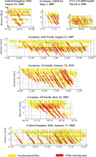
In 2000, Wilson used Gipp's model for simulating driver behavior on a ring road. In this case, every vehicle in the system is following another vehicle – the leader follows the last vehicle. The results of the experiment showed that the cars followed a free-flow time-space trajectory when the density on the ring road was low. However, as the number of vehicles on the road increases (density increases), kinematic waves begin to form as the congested part of the Gipps’ Model velocity equation prevails.

See also

• Newell's car-following model
• Intelligent driver model
• List of Runge–Kutta methods
• Simulation
• Traffic simulation

References

1. Spyropoulou, Ioanna (2007). "Simulation Using Gipps' Car-Following Model—An In-Depth Analysis". Transportmetrica. 3 (3): 231–245. doi:10.1080/18128600708685675. S2CID   111305074.
2. Wilson, R. E. (2001). "An analysis of Gipps' car-following model of highway traffic". IMA Journal of Applied Mathematics. 66 (5): 509–537. Bibcode:2001JApMa..66..509W. doi:10.1093/imamat/66.5.509.
3. Gipps, P. G. 1981 A behavioural car-following model for computer simulation. Transportation Research Part B, 15, 105-111

Further reading

• Bender, J. C. and Fendon R. E. (1972) On vehicles longitudinal dynamics. In Traffic Flow and Transportation, 19–32. Elsevier, New York.
• Gazis, D. C., Herman R. and Rothery R. W. (1961) Non-linear follow the leader models of traffic flow. Ops. Res. Vol. 9, 545–567.
• Gipps, P. G. (1976) Computer Program MULTSIM for Simulating Output from Vehicle Detectors on a Multi-Lane Signal Controlled Road. Transport Operations Research Group Working Paper No. 20, University of Newcastle-Upon-Tyne.
• Lee, G. (1966) A generalization of linear car-following theory. Ops. Res. Vol. 9, 209–229.
• Seddon, P. A. (1972) Program for simulating the dispersion of platoons in road traffic. Simulation Vol. 18, 81–90.