In econometrics, the autoregressive conditional heteroskedasticity (ARCH) model is a statistical model for time series data that describes the variance of the current error term or innovation as a function of the actual sizes of the previous time periods' error terms; often the variance is related to the squares of the previous innovations. The ARCH model is appropriate when the error variance in a time series follows an autoregressive (AR) model; if an autoregressive moving average (ARMA) model is assumed for the error variance, the model is a generalized autoregressive conditional heteroskedasticity (GARCH) model.

In statistics, the coefficient of determination, denoted R2 or r2 and pronounced "R squared", is the proportion of the variation in the dependent variable that is predictable from the independent variable(s).
In statistics, ordinary least squares (OLS) is a type of linear least squares method for choosing the unknown parameters in a linear regression model by the principle of least squares: minimizing the sum of the squares of the differences between the observed dependent variable in the input dataset and the output of the (linear) function of the independent variable. Some sources consider OLS to be linear regression.
Cointegration is a statistical property of a collection (X1, X2, ..., Xk) of time series variables. First, all of the series must be integrated of order d. Next, if a linear combination of this collection is integrated of order less than d, then the collection is said to be co-integrated. Formally, if (X,Y,Z) are each integrated of order d, and there exist coefficients a,b,c such that aX + bY + cZ is integrated of order less than d, then X, Y, and Z are cointegrated. Cointegration has become an important property in contemporary time series analysis. Time series often have trends—either deterministic or stochastic. In an influential paper, Charles Nelson and Charles Plosser (1982) provided statistical evidence that many US macroeconomic time series (like GNP, wages, employment, etc.) have stochastic trends.
In statistics, homogeneity and its opposite, heterogeneity, arise in describing the properties of a dataset, or several datasets. They relate to the validity of the often convenient assumption that the statistical properties of any one part of an overall dataset are the same as any other part. In meta-analysis, which combines the data from several studies, homogeneity measures the differences or similarities between the several studies.
In econometrics, the seemingly unrelated regressions (SUR) or seemingly unrelated regression equations (SURE) model, proposed by Arnold Zellner in (1962), is a generalization of a linear regression model that consists of several regression equations, each having its own dependent variable and potentially different sets of exogenous explanatory variables. Each equation is a valid linear regression on its own and can be estimated separately, which is why the system is called seemingly unrelated, although some authors suggest that the term seemingly related would be more appropriate, since the error terms are assumed to be correlated across the equations.
In statistics, the Breusch–Pagan test, developed in 1979 by Trevor Breusch and Adrian Pagan, is used to test for heteroskedasticity in a linear regression model. It was independently suggested with some extension by R. Dennis Cook and Sanford Weisberg in 1983. Derived from the Lagrange multiplier test principle, it tests whether the variance of the errors from a regression is dependent on the values of the independent variables. In that case, heteroskedasticity is present.
In statistics, semiparametric regression includes regression models that combine parametric and nonparametric models. They are often used in situations where the fully nonparametric model may not perform well or when the researcher wants to use a parametric model but the functional form with respect to a subset of the regressors or the density of the errors is not known. Semiparametric regression models are a particular type of semiparametric modelling and, since semiparametric models contain a parametric component, they rely on parametric assumptions and may be misspecified and inconsistent, just like a fully parametric model.
White test is a statistical test that establishes whether the variance of the errors in a regression model is constant: that is for homoskedasticity.
In statistics, the Ramsey Regression Equation Specification Error Test (RESET) test is a general specification test for the linear regression model. More specifically, it tests whether non-linear combinations of the explanatory variables help to explain the response variable. The intuition behind the test is that if non-linear combinations of the explanatory variables have any power in explaining the response variable, the model is misspecified in the sense that the data generating process might be better approximated by a polynomial or another non-linear functional form.
The topic of heteroskedasticity-consistent (HC) standard errors arises in statistics and econometrics in the context of linear regression and time series analysis. These are also known as heteroskedasticity-robust standard errors, Eicker–Huber–White standard errors, to recognize the contributions of Friedhelm Eicker, Peter J. Huber, and Halbert White.
In statistics, regression validation is the process of deciding whether the numerical results quantifying hypothesized relationships between variables, obtained from regression analysis, are acceptable as descriptions of the data. The validation process can involve analyzing the goodness of fit of the regression, analyzing whether the regression residuals are random, and checking whether the model's predictive performance deteriorates substantially when applied to data that were not used in model estimation.
An error correction model (ECM) belongs to a category of multiple time series models most commonly used for data where the underlying variables have a long-run common stochastic trend, also known as cointegration. ECMs are a theoretically-driven approach useful for estimating both short-term and long-term effects of one time series on another. The term error-correction relates to the fact that last-period's deviation from a long-run equilibrium, the error, influences its short-run dynamics. Thus ECMs directly estimate the speed at which a dependent variable returns to equilibrium after a change in other variables.

In statistics, the Goldfeld–Quandt test checks for heteroscedasticity in regression analyses. It does this by dividing a dataset into two parts or groups, and hence the test is sometimes called a two-group test. The Goldfeld–Quandt test is one of two tests proposed in a 1965 paper by Stephen Goldfeld and Richard Quandt. Both a parametric and nonparametric test are described in the paper, but the term "Goldfeld–Quandt test" is usually associated only with the former.
A Newey–West estimator is used in statistics and econometrics to provide an estimate of the covariance matrix of the parameters of a regression-type model where the standard assumptions of regression analysis do not apply. It was devised by Whitney K. Newey and Kenneth D. West in 1987, although there are a number of later variants. The estimator is used to try to overcome autocorrelation, and heteroskedasticity in the error terms in the models, often for regressions applied to time series data. The abbreviation "HAC," sometimes used for the estimator, stands for "heteroskedasticity and autocorrelation consistent." There are a number of HAC estimators described in, and HAC estimator does not refer uniquely to Newey–West. One version of Newey–West Bartlett requires the user to specify the bandwidth and usage of the Bartlett kernel from Kernel density estimation

Anil K. Bera is an Indian-American econometrician. He is Professor of Economics at University of Illinois at Urbana–Champaign's Department of Economics. He is most noted for his work with Carlos Jarque on the Jarque–Bera test.
In econometrics, the Park test is a test for heteroscedasticity. The test is based on the method proposed by Rolla Edward Park for estimating linear regression parameters in the presence of heteroscedastic error terms.
Control functions are statistical methods to correct for endogeneity problems by modelling the endogeneity in the error term. The approach thereby differs in important ways from other models that try to account for the same econometric problem. Instrumental variables, for example, attempt to model the endogenous variable X as an often invertible model with respect to a relevant and exogenous instrument Z. Panel analysis uses special data properties to difference out unobserved heterogeneity that is assumed to be fixed over time.
Richard T. Baillie is a British–American economist and statistician who is currently the A J Pasant Professor of Economics at the Michigan State University. He is also part time professor at King's College, London, and Senior Scientific Officer for the Rimini Center for Economic Analysis in Italy, and also on the Executive Council of the Society for Nonlinear Dynamics in Econometrics (SNDE).
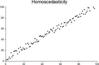
In statistics, a sequence of random variables is homoscedastic if all its random variables have the same finite variance; this is also known as homogeneity of variance. The complementary notion is called heteroscedasticity, also known as heterogeneity of variance. The spellings homoskedasticity and heteroskedasticity are also frequently used. “Skedasticity” comes from the Ancient Greek word “skedánnymi”, meaning “to scatter”. Assuming a variable is homoscedastic when in reality it is heteroscedastic results in unbiased but inefficient point estimates and in biased estimates of standard errors, and may result in overestimating the goodness of fit as measured by the Pearson coefficient.
