Background
In regression analysis, heteroscedasticity refers to unequal variances of the random error terms  , such that
 .
.
It is assumed that  . The above variance varies with
  , or the
  trial in an experiment or the case or observation in a dataset. Equivalently, heteroscedasticity refers to unequal conditional variances in the response variables
  , such that
 ,
,
again a value that depends on – or, more specifically, a value that is conditional on the values of one or more of the regressors  . Homoscedasticity, one of the basic Gauss–Markov assumptions of ordinary least squares linear regression modeling, refers to equal variance in the random error terms regardless of the trial or observation, such that
 , a constant.
Test description
Park, on noting a standard recommendation of assuming proportionality between error term variance and the square of the regressor, suggested instead that analysts 'assume a structure for the variance of the error term' and suggested one such structure: [1]

in which the error terms  are considered well behaved.
This relationship is used as the basis for this test.
The modeler first runs the unadjusted regression

where the latter contains p − 1 regressors, and then squares and takes the natural logarithm of each of the residuals ( ), which serve as estimators of the . The squared residuals
  in turn estimate
  .
.
If, then, in a regression of  on the natural logarithm of one or more of the regressors
  , we arrive at statistical significance for non-zero values on one or more of the
  , we reveal a connection between the residuals and the regressors. We reject the null hypothesis of homoscedasticity and conclude that heteroscedasticity is present.
In statistics, the Gauss–Markov theorem states that the ordinary least squares (OLS) estimator has the lowest sampling variance within the class of linear unbiased estimators, if the errors in the linear regression model are uncorrelated, have equal variances and expectation value of zero. The errors do not need to be normal, nor do they need to be independent and identically distributed. The requirement that the estimator be unbiased cannot be dropped, since biased estimators exist with lower variance. See, for example, the James–Stein estimator, ridge regression, or simply any degenerate estimator.
In statistics and optimization, errors and residuals are two closely related and easily confused measures of the deviation of an observed value of an element of a statistical sample from its "true value". The error of an observation is the deviation of the observed value from the true value of a quantity of interest. The residual is the difference between the observed value and the estimated value of the quantity of interest. The distinction is most important in regression analysis, where the concepts are sometimes called the regression errors and regression residuals and where they lead to the concept of studentized residuals. In econometrics, "errors" are also called disturbances.
In statistics, a studentized residual is the dimensionless ratio resulting from the division of a residual by an estimate of its standard deviation, both expressed in the same units. It is a form of a Student's t-statistic, with the estimate of error varying between points.
In econometrics, the autoregressive conditional heteroskedasticity (ARCH) model is a statistical model for time series data that describes the variance of the current error term or innovation as a function of the actual sizes of the previous time periods' error terms; often the variance is related to the squares of the previous innovations. The ARCH model is appropriate when the error variance in a time series follows an autoregressive (AR) model; if an autoregressive moving average (ARMA) model is assumed for the error variance, the model is a generalized autoregressive conditional heteroskedasticity (GARCH) model.

In statistics, ordinary least squares (OLS) is a type of linear least squares method for choosing the unknown parameters in a linear regression model by the principle of least squares: minimizing the sum of the squares of the differences between the observed dependent variable in the input dataset and the output of the (linear) function of the independent variable. Some sources consider OLS to be linear regression.
Weighted least squares (WLS), also known as weighted linear regression, is a generalization of ordinary least squares and linear regression in which knowledge of the unequal variance of observations (heteroscedasticity) is incorporated into the regression. WLS is also a specialization of generalized least squares, when all the off-diagonal entries of the covariance matrix of the errors, are null.
In statistics, simple linear regression (SLR) is a linear regression model with a single explanatory variable. That is, it concerns two-dimensional sample points with one independent variable and one dependent variable and finds a linear function that, as accurately as possible, predicts the dependent variable values as a function of the independent variable. The adjective simple refers to the fact that the outcome variable is related to a single predictor.
In econometrics, the seemingly unrelated regressions (SUR) or seemingly unrelated regression equations (SURE) model, proposed by Arnold Zellner in (1962), is a generalization of a linear regression model that consists of several regression equations, each having its own dependent variable and potentially different sets of exogenous explanatory variables. Each equation is a valid linear regression on its own and can be estimated separately, which is why the system is called seemingly unrelated, although some authors suggest that the term seemingly related would be more appropriate, since the error terms are assumed to be correlated across the equations.
In statistics, the Breusch–Pagan test, developed in 1979 by Trevor Breusch and Adrian Pagan, is used to test for heteroskedasticity in a linear regression model. It was independently suggested with some extension by R. Dennis Cook and Sanford Weisberg in 1983. Derived from the Lagrange multiplier test principle, it tests whether the variance of the errors from a regression is dependent on the values of the independent variables. In that case, heteroskedasticity is present.
In statistics the mean squared prediction error (MSPE), also known as mean squared error of the predictions, of a smoothing, curve fitting, or regression procedure is the expected value of the squared prediction errors (PE), the square difference between the fitted values implied by the predictive function and the values of the (unobservable) true value g. It is an inverse measure of the explanatory power of and can be used in the process of cross-validation of an estimated model. Knowledge of g would be required in order to calculate the MSPE exactly; in practice, MSPE is estimated.
In statistics, generalized least squares (GLS) is a method used to estimate the unknown parameters in a linear regression model. It is used when there is a non-zero amount of correlation between the residuals in the regression model. GLS is employed to improve statistical efficiency and reduce the risk of drawing erroneous inferences, as compared to conventional least squares and weighted least squares methods. It was first described by Alexander Aitken in 1935.
In statistics, Bayesian multivariate linear regression is a Bayesian approach to multivariate linear regression, i.e. linear regression where the predicted outcome is a vector of correlated random variables rather than a single scalar random variable. A more general treatment of this approach can be found in the article MMSE estimator.
The topic of heteroskedasticity-consistent (HC) standard errors arises in statistics and econometrics in the context of linear regression and time series analysis. These are also known as heteroskedasticity-robust standard errors, Eicker–Huber–White standard errors, to recognize the contributions of Friedhelm Eicker, Peter J. Huber, and Halbert White.
In statistics and in particular in regression analysis, leverage is a measure of how far away the independent variable values of an observation are from those of the other observations. High-leverage points, if any, are outliers with respect to the independent variables. That is, high-leverage points have no neighboring points in space, where is the number of independent variables in a regression model. This makes the fitted model likely to pass close to a high leverage observation. Hence high-leverage points have the potential to cause large changes in the parameter estimates when they are deleted i.e., to be influential points. Although an influential point will typically have high leverage, a high leverage point is not necessarily an influential point. The leverage is typically defined as the diagonal elements of the hat matrix.

In statistics, the Goldfeld–Quandt test checks for heteroscedasticity in regression analyses. It does this by dividing a dataset into two parts or groups, and hence the test is sometimes called a two-group test. The Goldfeld–Quandt test is one of two tests proposed in a 1965 paper by Stephen Goldfeld and Richard Quandt. Both a parametric and nonparametric test are described in the paper, but the term "Goldfeld–Quandt test" is usually associated only with the former.
A Newey–West estimator is used in statistics and econometrics to provide an estimate of the covariance matrix of the parameters of a regression-type model where the standard assumptions of regression analysis do not apply. It was devised by Whitney K. Newey and Kenneth D. West in 1987, although there are a number of later variants. The estimator is used to try to overcome autocorrelation, and heteroskedasticity in the error terms in the models, often for regressions applied to time series data. The abbreviation "HAC," sometimes used for the estimator, stands for "heteroskedasticity and autocorrelation consistent." There are a number of HAC estimators described in, and HAC estimator does not refer uniquely to Newey–West. One version of Newey–West Bartlett requires the user to specify the bandwidth and usage of the Bartlett kernel from Kernel density estimation

In statistics, errors-in-variables models or measurement error models are regression models that account for measurement errors in the independent variables. In contrast, standard regression models assume that those regressors have been measured exactly, or observed without error; as such, those models account only for errors in the dependent variables, or responses.
In statistics, the variance function is a smooth function that depicts the variance of a random quantity as a function of its mean. The variance function is a measure of heteroscedasticity and plays a large role in many settings of statistical modelling. It is a main ingredient in the generalized linear model framework and a tool used in non-parametric regression, semiparametric regression and functional data analysis. In parametric modeling, variance functions take on a parametric form and explicitly describe the relationship between the variance and the mean of a random quantity. In a non-parametric setting, the variance function is assumed to be a smooth function.
In statistics, the Glejser test for heteroscedasticity, developed in 1969 by Herbert Glejser, regresses the residuals on the explanatory variable that is thought to be related to the heteroscedastic variance. After it was found not to be asymptotically valid under asymmetric disturbances, similar improvements have been independently suggested by Im, and Machado and Santos Silva.
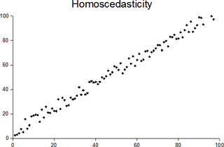
In statistics, a sequence of random variables is homoscedastic if all its random variables have the same finite variance; this is also known as homogeneity of variance. The complementary notion is called heteroscedasticity, also known as heterogeneity of variance. The spellings homoskedasticity and heteroskedasticity are also frequently used. “Skedasticity” comes from the Ancient Greek word “skedánnymi”, meaning “to scatter”. Assuming a variable is homoscedastic when in reality it is heteroscedastic results in unbiased but inefficient point estimates and in biased estimates of standard errors, and may result in overestimating the goodness of fit as measured by the Pearson coefficient.