A circle is a shape consisting of all points in a plane that are at a given distance from a given point, the centre. The distance between any point of the circle and the centre is called the radius. The length of a line segment connecting two points on the circle and passing through the centre is called the diameter. A circle bounds a region of the plane called a disc.
In complex analysis, an entire function, also called an integral function, is a complex-valued function that is holomorphic on the whole complex plane. Typical examples of entire functions are polynomials and the exponential function, and any finite sums, products and compositions of these, such as the trigonometric functions sine and cosine and their hyperbolic counterparts sinh and cosh, as well as derivatives and integrals of entire functions such as the error function. If an entire function has a root at , then , taking the limit value at , is an entire function. On the other hand, the natural logarithm, the reciprocal function, and the square root are all not entire functions, nor can they be continued analytically to an entire function.

A sphere is a geometrical object that is a three-dimensional analogue to a two-dimensional circle. Formally, a sphere is the set of points that are all at the same distance r from a given point in three-dimensional space. That given point is the center of the sphere, and r is the sphere's radius. The earliest known mentions of spheres appear in the work of the ancient Greek mathematicians.
In engineering, a transfer function of a system, sub-system, or component is a mathematical function that models the system's output for each possible input. It is widely used in electronic engineering tools like circuit simulators and control systems. In simple cases, this function can be represented as a two-dimensional graph of an independent scalar input versus the dependent scalar output. Transfer functions for components are used to design and analyze systems assembled from components, particularly using the block diagram technique, in electronics and control theory.

In mathematics, a stereographic projection is a perspective projection of the sphere, through a specific point on the sphere, onto a plane perpendicular to the diameter through the point. It is a smooth, bijective function from the entire sphere except the center of projection to the entire plane. It maps circles on the sphere to circles or lines on the plane, and is conformal, meaning that it preserves angles at which curves meet and thus locally approximately preserves shapes. It is neither isometric nor equiareal.

In electrical engineering and control theory, a Bode plot is a graph of the frequency response of a system. It is usually a combination of a Bode magnitude plot, expressing the magnitude of the frequency response, and a Bode phase plot, expressing the phase shift.

In mathematics, the complex plane is the plane formed by the complex numbers, with a Cartesian coordinate system such that the horizontal x-axis, called the real axis, is formed by the real numbers, and the vertical y-axis, called the imaginary axis, is formed by the imaginary numbers.

In geometry, the lemniscate of Bernoulli is a plane curve defined from two given points F1 and F2, known as foci, at distance 2c from each other as the locus of points P so that PF1·PF2 = c2. The curve has a shape similar to the numeral 8 and to the ∞ symbol. Its name is from lemniscatus, which is Latin for "decorated with hanging ribbons". It is a special case of the Cassini oval and is a rational algebraic curve of degree 4.

In control theory and stability theory, root locus analysis is a graphical method for examining how the roots of a system change with variation of a certain system parameter, commonly a gain within a feedback system. This is a technique used as a stability criterion in the field of classical control theory developed by Walter R. Evans which can determine stability of the system. The root locus plots the poles of the closed loop transfer function in the complex s-plane as a function of a gain parameter.

In geometry, a locus is a set of all points, whose location satisfies or is determined by one or more specified conditions.
In control theory and signal processing, a linear, time-invariant system is said to be minimum-phase if the system and its inverse are causal and stable.
Digital control is a branch of control theory that uses digital computers to act as system controllers. Depending on the requirements, a digital control system can take the form of a microcontroller to an ASIC to a standard desktop computer. Since a digital computer is a discrete system, the Laplace transform is replaced with the Z-transform. Since a digital computer has finite precision, extra care is needed to ensure the error in coefficients, analog-to-digital conversion, digital-to-analog conversion, etc. are not producing undesired or unplanned effects.
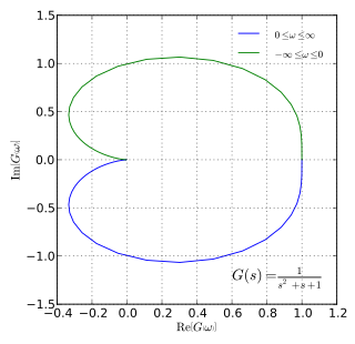
In control theory and stability theory, the Nyquist stability criterion or Strecker–Nyquist stability criterion, independently discovered by the German electrical engineer Felix Strecker at Siemens in 1930 and the Swedish-American electrical engineer Harry Nyquist at Bell Telephone Laboratories in 1932, is a graphical technique for determining the stability of a dynamical system.

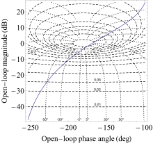
The Nichols plot is a plot used in signal processing and control design, named after American engineer Nathaniel B. Nichols. It plots the phase response versus the response magnitude of a transfer function for any given frequency, and as such is useful in characterizing a system's frequency response.
In mathematics, signal processing and control theory, a pole–zero plot is a graphical representation of a rational transfer function in the complex plane which helps to convey certain properties of the system such as:

In computing and mathematics, the function atan2 is the 2-argument arctangent. By definition, is the angle measure between the positive -axis and the ray from the origin to the point in the Cartesian plane. Equivalently, is the argument of the complex number

In mathematics, a complex logarithm is a generalization of the natural logarithm to nonzero complex numbers. The term refers to one of the following, which are strongly related:

In mathematics (particularly in complex analysis), the argument of a complex number z, denoted arg(z), is the angle between the positive real axis and the line joining the origin and z, represented as a point in the complex plane, shown as in Figure 1. By convention the positive real axis is drawn pointing rightward, the positive imaginary axis is drawn pointing upward, and complex numbers with positive real part are considered to have an anticlockwise argument with positive sign.
Iso-damping is a desirable system property referring to a state where the open-loop phase Bode plot is flat—i.e., the phase derivative with respect to the frequency is zero, at a given frequency called the "tangent frequency", . At the "tangent frequency" the Nyquist curve of the open-loop system tangentially touches the sensitivity circle and the phase Bode is locally flat which implies that the system will be more robust to gain variations. For systems that exhibit iso-damping property, the overshoots of the closed-loop step responses will remain almost constant for different values of the controller gain. This will ensure that the closed-loop system is robust to gain variations.
In control engineering, the sensitivity of a control system measures how variations in the plant parameters affects the closed-loop transfer function. Since the controller parameters are typically matched to the process characteristics and the process may change, it is important that the controller parameters are chosen in such a way that the closed loop system is not sensitive to variations in process dynamics. Moreover, the sensitivity function is also important to analyse how disturbances affects the system.
![Nyquist plot of the open-loop transfer function
G
(
s
)
=
1
/
(
s
+
0.5
)
{\displaystyle G(s)=1/(s+0.5)}
in blue with M and N circles overlaid in the plot. The M circle with M = 0.45 is highlighted in red and intercepts the Nyquist plot at frequencies
o
[?]
+-
1.64
{\displaystyle \omega \approx \pm 1.64}
. Nyquist grid.svg](http://upload.wikimedia.org/wikipedia/commons/thumb/b/b1/Nyquist_grid.svg/220px-Nyquist_grid.svg.png)