Joback method

Last updated

The Joback method [1] (often named Joback/Reid method) predicts eleven important and commonly used pure component thermodynamic properties from molecular structure only.

Contents

Basic principles

Group-contribution method

Principle of a group-contribution method Gruppenbeitragsmethodenprinzip.png
Principle of a group-contribution method

The Joback method is a group-contribution method. These kinds of methods use basic structural information of a chemical molecule, like a list of simple functional groups, add parameters to these functional groups, and calculate thermophysical and transport properties as a function of the sum of group parameters.

Joback assumes that there are no interactions between the groups, and therefore only uses additive contributions and no contributions for interactions between groups. Other group-contribution methods, especially methods like UNIFAC, which estimate mixture properties like activity coefficients, use both simple additive group parameters and group-interaction parameters. The big advantage of using only simple group parameters is the small number of needed parameters. The number of needed group-interaction parameters gets very high for an increasing number of groups (1 for two groups, 3 for three groups, 6 for four groups, 45 for ten groups and twice as much if the interactions are not symmetric).

Nine of the properties are single temperature-independent values, mostly estimated by a simple sum of group contribution plus an addend. Two of the estimated properties are temperature-dependent: the ideal-gas heat capacity and the dynamic viscosity of liquids. The heat-capacity polynomial uses 4 parameters, and the viscosity equation only 2. In both cases the equation parameters are calculated by group contributions.

History

The Joback method is an extension of the Lydersen method [2] and uses very similar groups, formulas, and parameters for the three properties the Lydersen already supported (critical temperature, critical pressure, critical volume).

Joback extended the range of supported properties, created new parameters and modified slightly the formulas of the old Lydersen method.

Model strengths and weaknesses

Strengths

The popularity and success of the Joback method mainly originates from the single group list for all properties. This allows one to get all eleven supported properties from a single analysis of the molecular structure.

The Joback method additionally uses a very simple and easy to assign group scheme, which makes the method usable for people with only basic chemical knowledge.

Weaknesses

Systematic errors of the Joback method (normal boiling point) JobackNormalBoilingPointSystematicError.png
Systematic errors of the Joback method (normal boiling point)

Newer developments of estimation methods [3] [4] have shown that the quality of the Joback method is limited. The original authors already stated themselves in the original article abstract: "High accuracy is not claimed, but the proposed methods are often as or more accurate than techniques in common use today."

The list of groups does not cover many common molecules sufficiently. Especially aromatic compounds are not differentiated from normal ring-containing components. This is a severe problem because aromatic and aliphatic components differ strongly.

The data base Joback and Reid used for obtaining the group parameters was rather small and covered only a limited number of different molecules. The best coverage has been achieved for normal boiling points (438 components), and the worst for heats of fusion (155 components). Current developments that can use data banks, like the Dortmund Data Bank or the DIPPR data base, have a much broader coverage.

The formula used for the prediction of the normal boiling point shows another problem. Joback assumed a constant contribution of added groups in homologous series like the alkanes. This doesn't describe the real behavior of the normal boiling points correctly. [5] Instead of the constant contribution, a decrease of the contribution with increasing number of groups must be applied. The chosen formula of the Joback method leads to high deviations for large and small molecules and an acceptable good estimation only for mid-sized components.

Formulas

In the following formulas Gi denotes a group contribution. Gi are counted for every single available group. If a group is present multiple times, each occurrence is counted separately.

Normal boiling point

Melting point

Critical temperature

This critical-temperature equation needs a normal boiling point Tb. If an experimental value is available, it is recommended to use this boiling point. It is, on the other hand, also possible to input the normal boiling point estimated by the Joback method. This will lead to a higher error.

Critical pressure

where Na is the number of atoms in the molecular structure (including hydrogens).

Critical volume

Heat of formation (ideal gas, 298 K)

Gibbs energy of formation (ideal gas, 298 K)

Heat capacity (ideal gas)

The Joback method uses a four-parameter polynomial to describe the temperature dependency of the ideal-gas heat capacity. These parameters are valid from 273 K to about 1000 K. But you are able to extend it to 1500K if you don't mind a bit of uncertainty here and there.

Heat of vaporization at normal boiling point

Heat of fusion

Liquid dynamic viscosity

where Mw is the molecular weight.

The method uses a two-parameter equation to describe the temperature dependency of the dynamic viscosity. The authors state that the parameters are valid from the melting temperature up to 0.7 of the critical temperature (Tr < 0.7).

Group contributions

GroupTcPcVcTbTmHformGformabcdHfusionHvapηaηb
Critical-state dataTemperatures
of phase transitions
Chemical caloric
properties
Ideal-gas heat capacitiesEnthalpies
of phase transitions
Dynamic viscosity
Non-ring groups
−CH30.0141−0.00126523.58−5.10−76.45−43.961.95E+1−8.08E−31.53E−4−9.67E−80.9082.373548.29−1.719
−CH20.01890.00005622.8811.27−20.648.42−9.09E−19.50E−2−5.44E−51.19E−82.5902.22694.16−0.199
>CH−0.01640.00204121.7412.6429.8958.36−2.30E+12.04E−1−2.65E−41.20E−70.7491.691−322.151.187
>C<0.00670.00432718.2546.4382.23116.02−6.62E+14.27E−1−6.41E−43.01E−7−1.4600.636−573.562.307
=CH20.0113−0.00285618.18−4.32−9.6303.772.36E+1−3.81E−21.72E−4−1.03E−7−0.4731.724495.01−1.539
=CH−0.0129−0.00064624.968.7337.9748.53−8.001.05E−1−9.63E−53.56E−82.6912.20582.28−0.242
=C<0.01170.00113824.1411.1483.9992.36−2.81E+12.08E−1−3.06E−41.46E−73.0632.138n. a.n. a.
=C=0.00260.00283626.1517.78142.14136.702.74E+1−5.57E−21.01E−4−5.02E−84.7202.661n. a.n. a.
≡CH0.0027−0.0008469.20−11.1879.3077.712.45E+1−2.71E−21.11E−4−6.78E−82.3221.155n. a.n. a.
≡C−0.00200.00163727.3864.32115.51109.827.872.01E−2−8.33E−61.39E-94.1513.302n. a.n. a.
Ring groups
−CH20.01000.00254827.157.75−26.80−3.68−6.038.54E−2−8.00E−6−1.80E−80.4902.398307.53−0.798
>CH−0.01220.00043821.7819.888.6740.99−2.05E+11.62E−1−1.60E−46.24E−83.2431.942−394.291.251
>C<0.00420.00612721.3260.1579.7287.88−9.09E+15.57E−1−9.00E−44.69E−7−1.3730.644n. a.n. a.
=CH−0.00820.00114126.738.132.0911.30−2.145.74E−2−1.64E−6−1.59E−81.1012.544259.65−0.702
=C<0.01430.00083231.0137.0246.4354.05−8.251.01E−1−1.42E−46.78E−82.3943.059-245.740.912
Halogen groups
−F0.0111−0.005727−0.03−15.78−251.92−247.192.65E+1−9.13E−21.91E−4−1.03E−71.398−0.670n. a.n. a.
−Cl0.0105−0.00495838.1313.55−71.55−64.313.33E+1−9.63E−21.87E−4−9.96E−82.5154.532625.45−1.814
−Br0.01330.00577166.8643.43−29.48−38.062.86E+1−6.49E−21.36E−4−7.45E−83.6036.582738.91−2.038
−I0.0068−0.00349793.8441.6921.065.743.21E+1−6.41E−21.26E−4−6.87E−82.7249.520809.55−2.224
Oxygen groups
−OH (alcohol)0.07410.01122892.8844.45−208.04−189.202.57E+1−6.91E−21.77E−4−9.88E−82.40616.8262173.72−5.057
−OH (phenol)0.02400.0184−2576.3482.83−221.65−197.37−2.811.11E−1−1.16E−44.94E−84.49012.4993018.17−7.314
−O− (non-ring)0.01680.00151822.4222.23−132.22−105.002.55E+1−6.32E−21.11E−4−5.48E−81.1882.410122.09−0.386
−O− (ring)0.00980.00481331.2223.05−138.16−98.221.22E+1−1.26E−26.03E−5−3.86E−85.8794.682440.24−0.953
>C=O (non-ring)0.03800.00316276.7561.20−133.22−120.506.456.70E−2−3.57E−52.86E−94.1898.972340.35−0.350
>C=O (ring)0.02840.00285594.9775.97−164.50−126.273.04E+1−8.29E−22.36E−4−1.31E−70.6.645n. a.n. a.
O=CH− (aldehyde)0.03790.00308272.2436.90−162.03−143.483.09E+1−3.36E−21.60E−4−9.88E−83.1979.093740.92−1.713
−COOH (acid)0.07910.007789169.09155.50−426.72−387.872.41E+14.27E−28.04E−5−6.87E−811.05119.5371317.23−2.578
−COO− (ester)0.04810.00058281.1053.60−337.92−301.952.45E+14.02E−24.02E−5−4.52E−86.9599.633483.88−0.966
=O (other than above)0.01430.010136−10.502.08−247.61−250.836.821.96E−21.27E−5−1.78E−83.6245.909675.24−1.340
Nitrogen groups
−NH20.02430.01093873.2366.89−22.0214.072.69E+1−4.12E−21.64E−4−9.76E−83.51510.788n. a.n. a.
>NH (non-ring)0.02950.00773550.1752.6653.4789.39−1.217.62E−2−4.86E−51.05E−85.0996.436n. a.n. a.
>NH (ring)0.01300.01142952.82101.5131.6575.611.18E+1−2.30E−21.07E−4−6.28E−87.4906.930n. a.n. a.
>N− (non-ring)0.01690.0074911.7448.84123.34163.16−3.11E+12.27E−1−3.20E−41.46E−74.7031.896n. a.n. a.
−N= (non-ring)0.0255-0.0099n. a.74.60n. a.23.61n. a.n. a.n. a.n. a.n. a.n. a.3.335n. a.n. a.
−N= (ring)0.00850.00763457.5568.4055.5279.938.83−3.84E-34.35E−5−2.60E−83.6496.528n. a.n. a.
=NHn. a.n. a.n. a.83.0868.9193.70119.665.69−4.12E−31.28E−4−8.88E−8n. a.12.169n. a.n. a.
−CN0.0496−0.010191125.6659.8988.4389.223.65E+1−7.33E−21.84E−4−1.03E−72.41412.851n. a.n. a.
−NO20.04370.006491152.54127.24−66.57−16.832.59E+1−3.74E−31.29E−4−8.88E−89.67916.738n. a.n. a.
Sulfur groups
−SH0.00310.00846363.5620.09−17.33−22.993.53E+1−7.58E−21.85E−4−1.03E−72.3606.884n. a.n. a.
−S− (non-ring)0.01190.00495468.7834.4041.8733.121.96E+1−5.61E−34.02E−5−2.76E−84.1306.817n. a.n. a.
−S− (ring)0.00190.00513852.1079.9339.1027.761.67E+14.81E−32.77E−5−2.11E−81.5575.984n. a.n. a.

Example calculation

AcetonGruppen.PNG

Acetone (propanone) is the simplest ketone and is separated into three groups in the Joback method: two methyl groups (−CH3) and one ketone group (C=O). Since the methyl group is present twice, its contributions have to be added twice.

−CH3>C=O (non-ring)
PropertyNo. of groupsGroup valueNo. of groupsGroup valueEstimated valueUnit
Tc
2
0.0141
1
0.0380
0.0662
500.5590
K
Pc
2
−1.20E−03
1
3.10E−03
7.00E−04
48.0250
bar
Vc
2
65.0000
1
62.0000
192.0000
209.5000
mL/mol
Tb
2
23.5800
1
76.7500
123.9100
322.1100
K
Tm
2
−5.1000
1
61.2000
51.0000
173.5000
K
Hformation
2
−76.4500
1
−133.2200
−286.1200
−217.8300
kJ/mol
Gformation
2
−43.9600
1
−120.5000
−208.4200
−154.5400
kJ/mol
Cp: a
2
1.95E+01
1
6.45E+00
4.55E+01
Cp: b
2
−8.08E−03
1
6.70E−02
5.08E−02
Cp: c
2
1.53E−04
1
−3.57E−05
2.70E−04
Cp: d
2
−9.67E−08
1
2.86E−09
−1.91E−07
Cp
at T = 300 K
75.3264
J/(mol·K)
Hfusion
2
0.9080
1
4.1890
6.0050
5.1250
kJ/mol
Hvap
2
2.3730
1
8.9720
13.7180
29.0180
kJ/mol
ηa
2
548.2900
1
340.3500
1436.9300
ηb
2
−1.7190
1
−0.3500
−3.7880
η
at T = 300 K
0.0002942
Pa·s

Related Research Articles

<span class="mw-page-title-main">Boiling point</span> Temperature at which a substance changes from liquid into vapor

The boiling point of a substance is the temperature at which the vapor pressure of a liquid equals the pressure surrounding the liquid and the liquid changes into a vapor.

<span class="mw-page-title-main">Enthalpy of vaporization</span> Energy to convert a liquid substance to a gas at a given pressure

In thermodynamics, the enthalpy of vaporization, also known as the (latent) heat of vaporization or heat of evaporation, is the amount of energy (enthalpy) that must be added to a liquid substance to transform a quantity of that substance into a gas. The enthalpy of vaporization is a function of the pressure and temperature at which the transformation takes place.

<span class="mw-page-title-main">Vapor pressure</span> Pressure exerted by a vapor in thermodynamic equilibrium

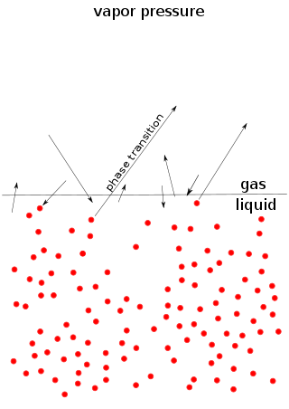
Vapor pressure or equilibrium vapor pressure is the pressure exerted by a vapor in thermodynamic equilibrium with its condensed phases at a given temperature in a closed system. The equilibrium vapor pressure is an indication of a liquid's thermodynamic tendency to evaporate. It relates to the balance of particles escaping from the liquid in equilibrium with those in a coexisting vapor phase. A substance with a high vapor pressure at normal temperatures is often referred to as volatile. The pressure exhibited by vapor present above a liquid surface is known as vapor pressure. As the temperature of a liquid increases, the attractive interactions between liquid molecules become less significant in comparison to the entropy of those molecules in the gas phase, increasing the vapor pressure. Thus, liquids with strong intermolecular interactions are likely to have smaller vapor pressures, with the reverse true for weaker interactions.

In chemistry, colligative properties are those properties of solutions that depend on the ratio of the number of solute particles to the number of solvent particles in a solution, and not on the nature of the chemical species present. The number ratio can be related to the various units for concentration of a solution such as molarity, molality, normality (chemistry), etc. The assumption that solution properties are independent of nature of solute particles is exact only for ideal solutions, which are solutions that exhibit thermodynamic properties analogous to those of an ideal gas, and is approximate for dilute real solutions. In other words, colligative properties are a set of solution properties that can be reasonably approximated by the assumption that the solution is ideal.

<span class="mw-page-title-main">Freezing-point depression</span> Process in which adding a solute to a solvent decreases the freezing point of the solvent

Freezing-point depression is a drop in the maximum temperature at which a substance freezes, caused when a smaller amount of another, non-volatile substance is added. Examples include adding salt into water, alcohol in water, ethylene or propylene glycol in water, adding copper to molten silver, or the mixing of two solids such as impurities into a finely powdered drug.

In statistics, a mixture model is a probabilistic model for representing the presence of subpopulations within an overall population, without requiring that an observed data set should identify the sub-population to which an individual observation belongs. Formally a mixture model corresponds to the mixture distribution that represents the probability distribution of observations in the overall population. However, while problems associated with "mixture distributions" relate to deriving the properties of the overall population from those of the sub-populations, "mixture models" are used to make statistical inferences about the properties of the sub-populations given only observations on the pooled population, without sub-population identity information. Mixture models are used for clustering, under the name model-based clustering, and also for density estimation.

<span class="mw-page-title-main">Critical point (thermodynamics)</span> Temperature and pressure point where phase boundaries disappear

In thermodynamics, a critical point is the end point of a phase equilibrium curve. One example is the liquid–vapor critical point, the end point of the pressure–temperature curve that designates conditions under which a liquid and its vapor can coexist. At higher temperatures, the gas cannot be liquefied by pressure alone. At the critical point, defined by a critical temperatureTc and a critical pressurepc, phase boundaries vanish. Other examples include the liquid–liquid critical points in mixtures, and the ferromagnet–paramagnet transition in the absence of an external magnetic field.

Rietveld refinement is a technique described by Hugo Rietveld for use in the characterisation of crystalline materials. The neutron and X-ray diffraction of powder samples results in a pattern characterised by reflections at certain positions. The height, width and position of these reflections can be used to determine many aspects of the material's structure.

In thermodynamics and chemical engineering, the vapor–liquid equilibrium (VLE) describes the distribution of a chemical species between the vapor phase and a liquid phase.

<span class="mw-page-title-main">UNIFAC</span> Liquid equilibrium model in statistical thermodynamics

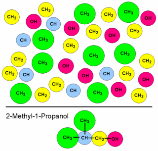
In statistical thermodynamics, the UNIFAC method is a semi-empirical system for the prediction of non-electrolyte activity in non-ideal mixtures. UNIFAC uses the functional groups present on the molecules that make up the liquid mixture to calculate activity coefficients. By using interactions for each of the functional groups present on the molecules, as well as some binary interaction coefficients, the activity of each of the solutions can be calculated. This information can be used to obtain information on liquid equilibria, which is useful in many thermodynamic calculations, such as chemical reactor design, and distillation calculations.

In statistical signal processing, the goal of spectral density estimation (SDE) or simply spectral estimation is to estimate the spectral density of a signal from a sequence of time samples of the signal. Intuitively speaking, the spectral density characterizes the frequency content of the signal. One purpose of estimating the spectral density is to detect any periodicities in the data, by observing peaks at the frequencies corresponding to these periodicities.

<span class="mw-page-title-main">UNIQUAC</span> Model of phase equilibrium in statistical thermodynamics

In statistical thermodynamics, UNIQUAC is an activity coefficient model used in description of phase equilibria. The model is a so-called lattice model and has been derived from a first order approximation of interacting molecule surfaces. The model is, however, not fully thermodynamically consistent due to its two-liquid mixture approach. In this approach the local concentration around one central molecule is assumed to be independent from the local composition around another type of molecule.

<span class="mw-page-title-main">Klincewicz method</span>

In thermodynamic theory, the Klincewicz method is a predictive method based both on group contributions and on a correlation with some basic molecular properties. The method estimates the critical temperature, the critical pressure, and the critical volume of pure components.

A group-contribution method in chemistry is a technique to estimate and predict thermodynamic and other properties from molecular structures.

PSRK is an estimation method for the calculation of phase equilibria of mixtures of chemical components. The original goal for the development of this method was to enable the estimation of properties of mixtures containing supercritical components. This class of substances cannot be predicted with established models, for example UNIFAC.

The Lydersen method is a group contribution method for the estimation of critical properties temperature (Tc), pressure (Pc) and volume (Vc). The Lydersen method is the prototype for and ancestor of many new models like Joback, Klincewicz, Ambrose, Gani-Constantinou and others.

<span class="mw-page-title-main">Enthalpy of fusion</span> Enthalpy change when a substance melts

In thermodynamics, the enthalpy of fusion of a substance, also known as (latent) heat of fusion, is the change in its enthalpy resulting from providing energy, typically heat, to a specific quantity of the substance to change its state from a solid to a liquid, at constant pressure.

MOSCED is a thermodynamic model for the estimation of limiting activity coefficients. From a historical point of view MOSCED can be regarded as an improved modification of the Hansen method and the Hildebrand solubility model by adding higher interaction term such as polarity, induction and separation of hydrogen bonding terms. This allows the prediction of polar and associative compounds, which most solubility parameter models have been found to do poorly. In addition to making quantitative prediction, MOSCED can be used to understand fundamental molecular level interaction for intuitive solvent selection and formulation.

VTPR is an estimation method for the calculation of phase equilibria of mixtures of chemical components. The original goal for the development of this method was to enable the estimation of properties of mixtures which contain supercritical components. These class of substances couldn't be predicted with established models like UNIFAC.

The shear viscosity of a fluid is a material property that describes the friction between internal neighboring fluid surfaces flowing with different fluid velocities. This friction is the effect of (linear) momentum exchange caused by molecules with sufficient energy to move between these fluid sheets due to fluctuations in their motion. The viscosity is not a material constant, but a material property that depends on temperature, pressure, fluid mixture composition, local velocity variations. This functional relationship is described by a mathematical viscosity model called a constitutive equation which is usually far more complex than the defining equation of shear viscosity. One such complicating feature is the relation between the viscosity model for a pure fluid and the model for a fluid mixture which is called mixing rules. When scientists and engineers use new arguments or theories to develop a new viscosity model, instead of improving the reigning model, it may lead to the first model in a new class of models. This article will display one or two representative models for different classes of viscosity models, and these classes are:

References

  1. Joback K. G., Reid R. C., "Estimation of Pure-Component Properties from Group-Contributions", Chem. Eng. Commun., 57, 233–243, 1987.
  2. Lydersen A. L., "Estimation of Critical Properties of Organic Compounds", University of Wisconsin College Engineering, Eng. Exp. Stn. Rep. 3, Madison, Wisconsin, 1955.
  3. Constantinou L., Gani R., "New Group Contribution Method for Estimating Properties of Pure Compounds", AIChE J., 40(10), 1697–1710, 1994.
  4. Nannoolal Y., Rarey J., Ramjugernath J., "Estimation of pure component properties Part 2. Estimation of critical property data by group contribution", Fluid Phase Equilib., 252(1–2), 1–27, 2007.
  5. Stein S. E., Brown R. L., "Estimation of Normal Boiling Points from Group Contributions", J. Chem. Inf. Comput. Sci. 34, 581–587 (1994).