Kernel regression

Not to be confused with Kernel principal component analysis or Kernel ridge regression.

In statistics, kernel regression is a non-parametric technique to estimate the conditional expectation of a random variable. The objective is to find a non-linear relation between a pair of random variables X and Y.

In any nonparametric regression, the conditional expectation of a variable ${\displaystyle Y}$ relative to a variable ${\displaystyle X}$ may be written:

${\displaystyle \operatorname {E} (Y\mid X)=m(X)}$

where ${\displaystyle m}$ is an unknown function.

Nadaraya–Watson kernel regression

Nadaraya and Watson, both in 1964, proposed to estimate ${\displaystyle m}$ as a locally weighted average, using a kernel as a weighting function. ^{[1] [2] [3]} The Nadaraya–Watson estimator is:

${\displaystyle {\widehat {m}}_{h}(x)={\frac {\sum _{i=1}^{n}K_{h}(x-x_{i})y_{i}}{\sum _{i=1}^{n}K_{h}(x-x_{i})}}}$

where ${\displaystyle K_{h}(t)={\frac {1}{h}}K\left({\frac {t}{h}}\right)}$ is a kernel with a bandwidth ${\displaystyle h}$ such that ${\displaystyle K(\cdot )}$ is of order at least 1, that is ${\displaystyle \int _{-\infty }^{\infty }uK(u)du=0}$.

Derivation

${\displaystyle \operatorname {E} (Y\mid X=x)=\int yf(y\mid x)\,dy=\int y{\frac {f(x,y)}{f(x)}}\,dy}$

Using the kernel density estimation for the joint distribution f(x,y) and f(x) with a kernel K,

${\displaystyle {\hat {f}}(x,y)={\frac {1}{n}}\sum _{i=1}^{n}K_{h}(x-x_{i})K_{h}(y-y_{i}),}$

${\displaystyle {\hat {f}}(x)={\frac {1}{n}}\sum _{i=1}^{n}K_{h}(x-x_{i}),}$

we get

${\displaystyle {\begin{aligned}\operatorname {\hat {E}} (Y\mid X=x)&=\int {\frac {y\sum _{i=1}^{n}K_{h}(x-x_{i})K_{h}(y-y_{i})}{\sum _{j=1}^{n}K_{h}(x-x_{j})}}\,dy,\\[6pt]&={\frac {\sum _{i=1}^{n}K_{h}(x-x_{i})\int y\,K_{h}(y-y_{i})\,dy}{\sum _{j=1}^{n}K_{h}(x-x_{j})}},\\[6pt]&={\frac {\sum _{i=1}^{n}K_{h}(x-x_{i})y_{i}}{\sum _{j=1}^{n}K_{h}(x-x_{j})}},\end{aligned}}}$

which is the Nadaraya–Watson estimator.

Priestley–Chao kernel estimator

${\displaystyle {\widehat {m}}_{PC}(x)=h^{-1}\sum _{i=2}^{n}(x_{i}-x_{i-1})K\left({\frac {x-x_{i}}{h}}\right)y_{i}}$

where ${\displaystyle h}$ is the bandwidth (or smoothing parameter).

Gasser–Müller kernel estimator ^[4]

${\displaystyle {\widehat {m}}_{GM}(x)=h^{-1}\sum _{i=1}^{n}\left[\int _{s_{i-1}}^{s_{i}}K\left({\frac {x-u}{h}}\right)\,du\right]y_{i}}$

where ${\displaystyle s_{i}={\frac {x_{i-1}+x_{i}}{2}}.}$

Example

Estimated regression function.

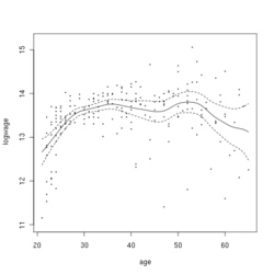
This example is based upon Canadian cross-section wage data consisting of a random sample taken from the 1971 Canadian Census Public Use Tapes for male individuals having common education (grade 13). There are 205 observations in total.^{[ citation needed ]}

The figure to the right shows the estimated regression function using a second order Gaussian kernel along with asymptotic variability bounds.

Script for example

The following commands of the R programming language use the npreg() function to deliver optimal smoothing and to create the figure given above. These commands can be entered at the command prompt via cut and paste.

install.packages("np")library(np)# non parametric librarydata(cps71)attach(cps71)m<-npreg(logwage~age)plot(m,plot.errors.method="asymptotic",plot.errors.style="band",ylim=c(11,15.2))points(age,logwage,cex=.25)detach(cps71)

Related

According to David Salsburg, the algorithms used in kernel regression were independently developed and used in fuzzy systems: "Coming up with almost exactly the same computer algorithm, fuzzy systems and kernel density-based regressions appear to have been developed completely independently of one another." ^[5]

Statistical implementation

• GNU Octave mathematical program package
• Julia: KernelEstimator.jl
• MATLAB: A free MATLAB toolbox with implementation of kernel regression, kernel density estimation, kernel estimation of hazard function and many others is available on these pages (this toolbox is a part of the book ^[6] ).
• Python: the KernelReg class for mixed data types in the statsmodels.nonparametric sub-package (includes other kernel density related classes), the package kernel_regression as an extension of scikit-learn (inefficient memory-wise, useful only for small datasets)
• R: the function npreg of the np package can perform kernel regression. ^{[7] [8]}
• Stata: npregress, kernreg2

See also

• Kernel smoother
• Local regression

References

1. Nadaraya, E. A. (1964). "On Estimating Regression". Theory of Probability and Its Applications. 9 (1): 141–2. doi:10.1137/1109020.
2. Watson, G. S. (1964). "Smooth regression analysis". Sankhyā: The Indian Journal of Statistics, Series A. 26 (4): 359–372. JSTOR   25049340.
3. Bierens, Herman J. (1994). "The Nadaraya–Watson kernel regression function estimator". Topics in Advanced Econometrics. New York: Cambridge University Press. pp. 212–247. ISBN   0-521-41900-X.
4. Gasser, Theo; Müller, Hans-Georg (1979). "Kernel estimation of regression functions". Springer: 23–68.
5. Salsburg, D. (2002). The Lady Tasting Tea: How Statistics Revolutionized Science in the Twentieth Century . W.H. Freeman. pp. 290–91. ISBN   0-8050-7134-2.
6. Horová, I.; Koláček, J.; Zelinka, J. (2012). Kernel Smoothing in MATLAB: Theory and Practice of Kernel Smoothing. Singapore: World Scientific Publishing. ISBN   978-981-4405-48-5.
7. np: Nonparametric kernel smoothing methods for mixed data types
8. Kloke, John; McKean, Joseph W. (2014). Nonparametric Statistical Methods Using R. CRC Press. pp. 98–106. ISBN   978-1-4398-7343-4.

Further reading

• Henderson, Daniel J.; Parmeter, Christopher F. (2015). Applied Nonparametric Econometrics. Cambridge University Press. ISBN   978-1-107-01025-3.
• Li, Qi; Racine, Jeffrey S. (2007). Nonparametric Econometrics: Theory and Practice. Princeton University Press. ISBN   978-0-691-12161-1.
• Pagan, A.; Ullah, A. (1999). Nonparametric Econometrics . Cambridge University Press. ISBN   0-521-35564-8.
• Racine, Jeffrey S. (2019). An Introduction to the Advanced Theory and Practice of Nonparametric Econometrics: A Replicable Approach Using R. Cambridge University Press. ISBN   9781108483407.
• Simonoff, Jeffrey S. (1996). Smoothing Methods in Statistics. Springer. ISBN   0-387-94716-7.

External links

• Scale-adaptive kernel regression (with Matlab software).
• Tutorial of Kernel regression using spreadsheet (with Microsoft Excel).
• An online kernel regression demonstration Requires .NET 3.0 or later.
• Kernel regression with automatic bandwidth selection (with Python)