Level ancestor problem

Last updated

In graph theory and theoretical computer science, the level ancestor problem is the problem of preprocessing a given rooted tree T into a data structure that can determine the ancestor of a given node at a given distance from the root of the tree.

Contents

More precisely, let T be a rooted tree with n nodes, and let v be an arbitrary node of T. The level ancestor query LA(v,d) requests the ancestor of node v at depth d, where the depth of a node v in a tree is the number of edges on the shortest path from the root of the tree to node v. It is possible to solve this problem in constant time per query, after a preprocessing algorithm that takes O(n) and that builds a data structure that uses O(n) storage space. [1] [2]

Naive methods

Level ancestor of (v,2) and the path from root r to the node v. LevelAncestor.png
Level ancestor of (v,2) and the path from root r to the node v.

The simplest way to find a level ancestor of a node is to climb up the tree towards the root of the tree. On the path to the root of the tree, every ancestor of a node can be visited and therefore reported. In this case, the tree does not need to be preprocessed and the time to answer a query is O(h), where "h" is the height of the tree. This approach is not feasible in situations where the tree may have large height and a large number of a queries are required to be processed.

Alternatively, all the possible solutions can be precomputed and stored in a table. In this case, the queries can be answered in O(1) but the space and the preprocessing time is O(n2).

The simplest queries that can be answered in constant time without any preprocessing are LA(v, 0) and LA(v, depth(v)). In the former case, the answer is always the root of the tree and in the latter case, the answer is the node v itself. Each of these results takes O(1).

Storing the paths through the tree in a skew binary random access list allows the tree to still be extended downward one O(1) step at a time, but now allows the search to proceed in O(log(p)), where "p" is the distance from v to the requested depth. This approach is feasible when the tree is particularly wide or will be extended online and so can't be effectively preprocessed, as the storage and access time is purely determined by path length. [3]

Jump pointer algorithm

The jump pointer algorithm [1] pre-processes a tree in O(n log n) time and answers level ancestor queries in O(log n) time. The jump pointer algorithm associates up to log n pointers to each vertex of the tree. These pointers are called jump pointers because they jump up the tree towards the root of the tree. For a given node v of a tree, the algorithm stores an array of length jumpers where . The ith element of this array points to the 2ith ancestor of v. Using such data structure helps us jump halfway up the tree from any given node. When the algorithm is asked to process a query, we repeatedly jump up the tree using these pointers. The number of jumps will be at most log n and therefore queries can be answered in log n time.

Ladder algorithm

The ladder algorithm [1] is based on the idea of simplifying a tree into a collection of paths. The reason for this is the fact that paths are easier to be queried when it comes to level ancestor queries. Consider a path P consisting of n nodes rooted at a node r. We can store the path into an array of size n called Ladder and we can quickly answer a level ancestor query of LA(v, d) by returning Ladder[d] if depth(v)≤d. This will take O(1). However, this will only work if the given tree is a path. Otherwise, we need to decompose it into paths. This is done in two stages: long-path decomposition and extending the long paths into ladders.

Stage 1: long-path decomposition

This is a recursive method that decomposes a given tree into paths. This stages starts off by finding the longest root-to-leaf path in the tree. It then removes this path by breaking its ties from the tree which will break the remaining of the tree into sub-trees and then it recursively processes each sub-tree. Every time a path is decomposed, an array is created in association with the path that contains the elements on the path from the root to the leaf. The base case of this recursion is when the tree is a path in which case its removal leaves an empty graph. Each vertex v has a unique ladder which is the ladder containing it and we call it the "v's ladder". However, after this pre-processing stage, the queries cannot be answered quickly. In fact in order to answer a level ancestor query, the algorithm needs to jump from a path to another until it reaches the root and there could be Θ(n) of such paths on a leaf-to-root path. This leads us to an algorithm that can pre-process the tree in O(n) time and answers queries in O(n). In order to reach the optimal query time, we need to process the results in a second stage described below.

Stage 2: extending the long paths into ladders

The first stage of the algorithm decomposes the tree into a number of disjoint paths. In the second stage of the algorithm, each path is extended and therefore the resulting paths will not be mutually exclusive. In the first stage of the algorithm, each path is associated with an array of size h' . We extend this path by adding the h' immediate ancestors at the top of the path in the same array. This will extend each array twice its original size at most which will result in 2n total number of nodes in all the ladders. Notice that the number of ladders is not changed and each node's ladder remains the same. Although a node v can be listed in multiple paths now but its ladder is the one that was associated to v in the first stage of the algorithm. These two stages can be processes in O(n) but the query time is not constant yet. Consider a level ancestor query on a node u of height h. By travelling to the top of u's ladder, a vertex of height at least 2h will be reached. Observe that all the nodes have a height of at least 1 and therefore after doing this i times, we reach a node of height at least 2i and therefore we need to do this at most log n times. This gives us a query time of O(log n).

Stage 3: combining the two approaches

It turns out that the ladder algorithm does not do the trick on its own. In fact the jump pointer algorithm and the ladder algorithm complement one another. The two algorithms work in opposite directions: the jump pointer algorithm makes exponentially decreasing hops and the ladder algorithm makes exponentially increasing hops. A combination of the two algorithms can answer queries in O(1) time. A single jump pointer takes any query at least halfway up the tree after which climbing up only one ladder will answer the query. This results in O(n log n) pre-processing time and O(1) query time. The pre-processing can be further reduced to O(n) time by an application of the Method of Four Russians, in which the tree is reduced to a smaller tree with linear preprocessing, and a collection of very small trees, which are small enough that an exhaustive enumeration of all trees and the preprocessing of those trees is still O(n) time. Trees of size (log n)/4 suffice.

Berkman and Vishkin's solution

A different solution is due to Berkman and Vishkin. [2] [4] This solution is based on the Euler tour technique for processing trees. The main observation is that LA(v,d) is the first node of depth d that appears in the Euler tour after the last appearance of v. Thus, by constructing the Euler tour and associated information on depth, the problem is reduced to a query on arrays, named find smaller (FS). For an array A, and a valid index i, FS(i,x) returns the first index j>i such that A[i]<x (here, we use x=d+1). An efficient solution to the FS problem is hard in general, but easier for the special case that arises from Euler tours; in this case, adjacent elements differ by ±1. This idea yields O(1) query time, with a preprocessing algorithm of complexity O(n log n). The preprocessing time is improved to O(n) by an application of the Method of Four Russians.

See also

Related Research Articles

Binary search algorithm Search algorithm finding the position of a target value within a sorted array

In computer science, binary search, also known as half-interval search, logarithmic search, or binary chop, is a search algorithm that finds the position of a target value within a sorted array. Binary search compares the target value to the middle element of the array. If they are not equal, the half in which the target cannot lie is eliminated and the search continues on the remaining half, again taking the middle element to compare to the target value, and repeating this until the target value is found. If the search ends with the remaining half being empty, the target is not in the array.

In computer science, a red–black tree is a kind of self-balancing binary search tree. Each node stores an extra bit representing "color", used to ensure that the tree remains balanced during insertions and deletions.

The point location problem is a fundamental topic of computational geometry. It finds applications in areas that deal with processing geometrical data: computer graphics, geographic information systems (GIS), motion planning, and computer aided design (CAD).

Quadtree Tree data structure in which each internal node has exactly four children, to partition a 2D area

A quadtree is a tree data structure in which each internal node has exactly four children. Quadtrees are the two-dimensional analog of octrees and are most often used to partition a two-dimensional space by recursively subdividing it into four quadrants or regions. The data associated with a leaf cell varies by application, but the leaf cell represents a "unit of interesting spatial information".

In computer science, tree traversal is a form of graph traversal and refers to the process of visiting each node in a tree data structure, exactly once. Such traversals are classified by the order in which the nodes are visited. The following algorithms are described for a binary tree, but they may be generalized to other trees as well.

In computing, a persistent data structure or not ephemeral data structure is a data structure that always preserves the previous version of itself when it is modified. Such data structures are effectively immutable, as their operations do not (visibly) update the structure in-place, but instead always yield a new updated structure. The term was introduced in Driscoll, Sarnak, Sleator, and Tarjans' 1986 article.

In computer science, a disjoint-set data structure, also called a union–find data structure or merge–find set, is a data structure that stores a collection of disjoint (non-overlapping) sets. Equivalently, it stores a partition of a set into disjoint subsets. It provides operations for adding new sets, merging sets, and finding a representative member of a set. The last operation allows to find out efficiently if any two elements are in the same or different sets.

In computer science, an interval tree is a tree data structure to hold intervals. Specifically, it allows one to efficiently find all intervals that overlap with any given interval or point. It is often used for windowing queries, for instance, to find all roads on a computerized map inside a rectangular viewport, or to find all visible elements inside a three-dimensional scene. A similar data structure is the segment tree.

<i>m</i>-ary tree

In graph theory, an m-ary tree is a rooted tree in which each node has no more than m children. A binary tree is the special case where m = 2, and a ternary tree is another case with m = 3 that limits its children to three.

In graph theory and computer science, the lowest common ancestor (LCA) of two nodes v and w in a tree or directed acyclic graph (DAG) T is the lowest node that has both v and w as descendants, where we define each node to be a descendant of itself.

A link/cut tree is a data structure for representing a forest, a set of rooted trees, and offers the following operations:

Cartesian tree

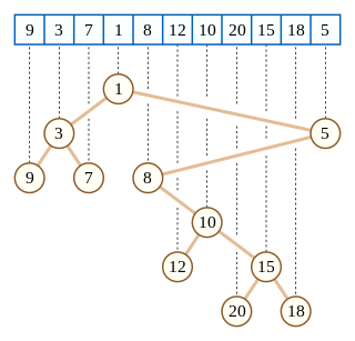
In computer science, a Cartesian tree is a binary tree derived from a sequence of numbers; it can be uniquely defined from the properties that it is heap-ordered and that a symmetric (in-order) traversal of the tree returns the original sequence. Introduced by Vuillemin (1980) in the context of geometric range searching data structures, Cartesian trees have also been used in the definition of the treap and randomized binary search tree data structures for binary search problems. The Cartesian tree for a sequence may be constructed in linear time using a stack-based algorithm for finding all nearest smaller values in a sequence.

Range minimum query Minimizing problem in computer programming

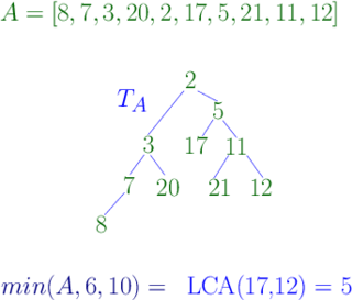
In computer science, a range minimum query (RMQ) solves the problem of finding the minimal value in a sub-array of an array of comparable objects. Range minimum queries have several use cases in computer science, such as the lowest common ancestor problem and the longest common prefix problem (LCP).

Euler tour technique

The Euler tour technique (ETT), named after Leonhard Euler, is a method in graph theory for representing trees. The tree is viewed as a directed graph that contains two directed edges for each edge in the tree. The tree can then be represented as a Eulerian circuit of the directed graph, known as the Euler tour representation (ETR) of the tree. The ETT allows for efficient, parallel computation of solutions to common problems in algorithmic graph theory. It was introduced by Tarjan and Vishkin in 1984.

In computer science, an x-fast trie is a data structure for storing integers from a bounded domain. It supports exact and predecessor or successor queries in time O(log log M), using O(n log M) space, where n is the number of stored values and M is the maximum value in the domain. The structure was proposed by Dan Willard in 1982, along with the more complicated y-fast trie, as a way to improve the space usage of van Emde Boas trees, while retaining the O(log log M) query time.

In data structures, a range query consists of preprocessing some input data into a data structure to efficiently answer any number of queries on any subset of the input. Particularly, there is a group of problems that have been extensively studied where the input is an array of unsorted numbers and a query consists of computing some function, such as the minimum, on a specific range of the array.

In computer science, the longest common prefix array is an auxiliary data structure to the suffix array. It stores the lengths of the longest common prefixes (LCPs) between all pairs of consecutive suffixes in a sorted suffix array.

Pointer jumping or path doubling is a design technique for parallel algorithms that operate on pointer structures, such as linked lists and directed graphs. Pointer jumping allows an algorithm to follow paths with a time complexity that is logarithmic with respect to the length of the longest path. It does this by "jumping" to the end of the path computed by neighbors.

In computer science, k-way merge algorithms or multiway merges are a specific type of sequence merge algorithms that specialize in taking in k sorted lists and merging them into a single sorted list. These merge algorithms generally refer to merge algorithms that take in a number of sorted lists greater than two. Two-way merges are also referred to as binary merges.

In computer science, a weak heap is a data structure for priority queues, combining features of the binary heap and binomial heap. It can be stored in an array as an implicit binary tree like a binary heap, and has the efficiency guarantees of binomial heaps.

References

  1. 1 2 3 Bender, Michael A.; Farach-Colton, Martin (2004). "The Level Ancestor Problem Simplified". Theor. Comput. Sci. 321: 5–12. doi: 10.1016/j.tcs.2003.05.002 .
  2. 1 2 Berkman, Omer; Vishkin, Uzi (Apr 1994). "Finding level-ancestors in trees". J. Comput. Syst. Sci. 2. 48 (2): 214–230. doi: 10.1016/S0022-0000(05)80002-9 .
  3. Kmett, Edward. "O(log n) persistent on-line lowest common ancestor calculation without preprocessing" . Retrieved 8 May 2013.
  4. Ben-Amram, Amir M. (2009). "The Euler Path to Static Level-Ancestors". arXiv: 0909.1030v1 [cs.DS].