A likelihood function measures how well a statistical model explains observed data by calculating the probability of seeing that data under different parameter values of the model. It is constructed from the joint probability distribution of the random variable that (presumably) generated the observations. When evaluated on the actual data points, it becomes a function solely of the model parameters.

In probability theory and statistics, the multivariate normal distribution, multivariate Gaussian distribution, or joint normal distribution is a generalization of the one-dimensional (univariate) normal distribution to higher dimensions. One definition is that a random vector is said to be k-variate normally distributed if every linear combination of its k components has a univariate normal distribution. Its importance derives mainly from the multivariate central limit theorem. The multivariate normal distribution is often used to describe, at least approximately, any set of (possibly) correlated real-valued random variables, each of which clusters around a mean value.

The method of least squares is a parameter estimation method in regression analysis based on minimizing the sum of the squares of the residuals made in the results of each individual equation.

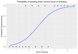
In statistics, the logistic model is a statistical model that models the log-odds of an event as a linear combination of one or more independent variables. In regression analysis, logistic regression estimates the parameters of a logistic model. In binary logistic regression there is a single binary dependent variable, coded by an indicator variable, where the two values are labeled "0" and "1", while the independent variables can each be a binary variable or a continuous variable. The corresponding probability of the value labeled "1" can vary between 0 and 1, hence the labeling; the function that converts log-odds to probability is the logistic function, hence the name. The unit of measurement for the log-odds scale is called a logit, from logistic unit, hence the alternative names. See § Background and § Definition for formal mathematics, and § Example for a worked example.
In statistics, a generalized linear model (GLM) is a flexible generalization of ordinary linear regression. The GLM generalizes linear regression by allowing the linear model to be related to the response variable via a link function and by allowing the magnitude of the variance of each measurement to be a function of its predicted value.

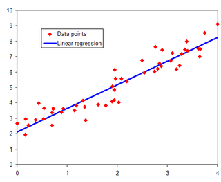
In statistical modeling, regression analysis is a set of statistical processes for estimating the relationships between a dependent variable and one or more error-free independent variables. The most common form of regression analysis is linear regression, in which one finds the line that most closely fits the data according to a specific mathematical criterion. For example, the method of ordinary least squares computes the unique line that minimizes the sum of squared differences between the true data and that line. For specific mathematical reasons, this allows the researcher to estimate the conditional expectation of the dependent variable when the independent variables take on a given set of values. Less common forms of regression use slightly different procedures to estimate alternative location parameters or estimate the conditional expectation across a broader collection of non-linear models.
In mathematics and computing, the Levenberg–Marquardt algorithm, also known as the damped least-squares (DLS) method, is used to solve non-linear least squares problems. These minimization problems arise especially in least squares curve fitting. The LMA interpolates between the Gauss–Newton algorithm (GNA) and the method of gradient descent. The LMA is more robust than the GNA, which means that in many cases it finds a solution even if it starts very far off the final minimum. For well-behaved functions and reasonable starting parameters, the LMA tends to be slower than the GNA. LMA can also be viewed as Gauss–Newton using a trust region approach.
Weighted least squares (WLS), also known as weighted linear regression, is a generalization of ordinary least squares and linear regression in which knowledge of the unequal variance of observations (heteroscedasticity) is incorporated into the regression. WLS is also a specialization of generalized least squares, when all the off-diagonal entries of the covariance matrix of the errors, are null.
In statistics, generalized least squares (GLS) is a method used to estimate the unknown parameters in a linear regression model. It is used when there is a non-zero amount of correlation between the residuals in the regression model. GLS is employed to improve statistical efficiency and reduce the risk of drawing erroneous inferences, as compared to conventional least squares and weighted least squares methods. It was first described by Alexander Aitken in 1935.
The cross-entropy (CE) method is a Monte Carlo method for importance sampling and optimization. It is applicable to both combinatorial and continuous problems, with either a static or noisy objective.
Uncertainty quantification (UQ) is the science of quantitative characterization and estimation of uncertainties in both computational and real world applications. It tries to determine how likely certain outcomes are if some aspects of the system are not exactly known. An example would be to predict the acceleration of a human body in a head-on crash with another car: even if the speed was exactly known, small differences in the manufacturing of individual cars, how tightly every bolt has been tightened, etc., will lead to different results that can only be predicted in a statistical sense.
Bayesian linear regression is a type of conditional modeling in which the mean of one variable is described by a linear combination of other variables, with the goal of obtaining the posterior probability of the regression coefficients and ultimately allowing the out-of-sample prediction of the regressandconditional on observed values of the regressors. The simplest and most widely used version of this model is the normal linear model, in which given is distributed Gaussian. In this model, and under a particular choice of prior probabilities for the parameters—so-called conjugate priors—the posterior can be found analytically. With more arbitrarily chosen priors, the posteriors generally have to be approximated.

Probabilistic design is a discipline within engineering design. It deals primarily with the consideration and minimization of the effects of random variability upon the performance of an engineering system during the design phase. Typically, these effects studied and optimized are related to quality and reliability. It differs from the classical approach to design by assuming a small probability of failure instead of using the safety factor. Probabilistic design is used in a variety of different applications to assess the likelihood of failure. Disciplines which extensively use probabilistic design principles include product design, quality control, systems engineering, machine design, civil engineering and manufacturing.
Non-linear least squares is the form of least squares analysis used to fit a set of m observations with a model that is non-linear in n unknown parameters (m ≥ n). It is used in some forms of nonlinear regression. The basis of the method is to approximate the model by a linear one and to refine the parameters by successive iterations. There are many similarities to linear least squares, but also some significant differences. In economic theory, the non-linear least squares method is applied in (i) the probit regression, (ii) threshold regression, (iii) smooth regression, (iv) logistic link regression, (v) Box–Cox transformed regressors ().
Linear least squares (LLS) is the least squares approximation of linear functions to data. It is a set of formulations for solving statistical problems involved in linear regression, including variants for ordinary (unweighted), weighted, and generalized (correlated) residuals. Numerical methods for linear least squares include inverting the matrix of the normal equations and orthogonal decomposition methods.
Probability bounds analysis (PBA) is a collection of methods of uncertainty propagation for making qualitative and quantitative calculations in the face of uncertainties of various kinds. It is used to project partial information about random variables and other quantities through mathematical expressions. For instance, it computes sure bounds on the distribution of a sum, product, or more complex function, given only sure bounds on the distributions of the inputs. Such bounds are called probability boxes, and constrain cumulative probability distributions.
Subset simulation is a method used in reliability engineering to compute small failure probabilities encountered in engineering systems. The basic idea is to express a small failure probability as a product of larger conditional probabilities by introducing intermediate failure events. This conceptually converts the original rare-event problem into a series of frequent-event problems that are easier to solve. In the actual implementation, samples conditional on intermediate failure events are adaptively generated to gradually populate from the frequent to rare event region. These 'conditional samples' provide information for estimating the complementary cumulative distribution function (CCDF) of the quantity of interest, covering the high as well as the low probability regions. They can also be used for investigating the cause and consequence of failure events. The generation of conditional samples is not trivial but can be performed efficiently using Markov chain Monte Carlo (MCMC).
In statistics, linear regression is a model that estimates the linear relationship between a scalar response and one or more explanatory variables. A model with exactly one explanatory variable is a simple linear regression; a model with two or more explanatory variables is a multiple linear regression. This term is distinct from multivariate linear regression, which predicts multiple correlated dependent variables rather than a single dependent variable.
In regression analysis, an interval predictor model (IPM) is an approach to regression where bounds on the function to be approximated are obtained. This differs from other techniques in machine learning, where usually one wishes to estimate point values or an entire probability distribution. Interval Predictor Models are sometimes referred to as a nonparametric regression technique, because a potentially infinite set of functions are contained by the IPM, and no specific distribution is implied for the regressed variables.

The hyperbolastic functions, also known as hyperbolastic growth models, are mathematical functions that are used in medical statistical modeling. These models were originally developed to capture the growth dynamics of multicellular tumor spheres, and were introduced in 2005 by Mohammad Tabatabai, David Williams, and Zoran Bursac. The precision of hyperbolastic functions in modeling real world problems is somewhat due to their flexibility in their point of inflection. These functions can be used in a wide variety of modeling problems such as tumor growth, stem cell proliferation, pharma kinetics, cancer growth, sigmoid activation function in neural networks, and epidemiological disease progression or regression.


