In computational mathematics, an iterative method is a mathematical procedure that uses an initial value to generate a sequence of improving approximate solutions for a class of problems, in which the n-th approximation is derived from the previous ones. A specific implementation of an iterative method, including the termination criteria, is an algorithm of the iterative method. An iterative method is called convergent if the corresponding sequence converges for given initial approximations. A mathematically rigorous convergence analysis of an iterative method is usually performed; however, heuristic-based iterative methods are also common.

In mathematics, particularly linear algebra and numerical analysis, the Gram–Schmidt process is a method for orthonormalizing a set of vectors in an inner product space, most commonly the Euclidean space Rn equipped with the standard inner product. The Gram–Schmidt process takes a finite, linearly independent set of vectors S = {v1, ..., vk} for k ≤ n and generates an orthogonal set S′ = {u1, ..., uk} that spans the same k-dimensional subspace of Rn as S.
In Riemannian geometry, the sectional curvature is one of the ways to describe the curvature of Riemannian manifolds with dimension greater than 1. The sectional curvature K(σp) depends on a two-dimensional linear subspace σp of the tangent space at a point p of the manifold. It can be defined geometrically as the Gaussian curvature of the surface which has the plane σp as a tangent plane at p, obtained from geodesics which start at p in the directions of σp. The sectional curvature is a real-valued function on the 2-Grassmannian bundle over the manifold.
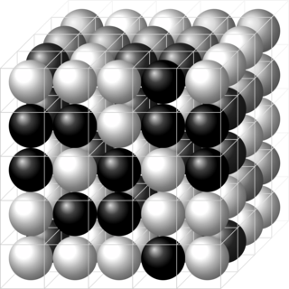
In physics, a lattice model is a physical model that is defined on a lattice, as opposed to the continuum of space or spacetime. Lattice models originally occurred in the context of condensed matter physics, where the atoms of a crystal automatically form a lattice. Currently, lattice models are quite popular in theoretical physics, for many reasons. Some models are exactly solvable, and thus offer insight into physics beyond what can be learned from perturbation theory. Lattice models are also ideal for study by the methods of computational physics, as the discretization of any continuum model automatically turns it into a lattice model. The exact solution to many of these models includes the presence of solitons. Techniques for solving these include the inverse scattering transform and the method of Lax pairs, the Yang–Baxter equation and quantum groups. The solution of these models has given insights into the nature of phase transitions, magnetization and scaling behaviour, as well as insights into the nature of quantum field theory. Physical lattice models frequently occur as an approximation to a continuum theory, either to give an ultraviolet cutoff to the theory to prevent divergences or to perform numerical computations. An example of a continuum theory that is widely studied by lattice models is the QCD lattice model, a discretization of quantum chromodynamics. However, digital physics considers nature fundamentally discrete at the Planck scale, which imposes upper limit to the density of information, aka Holographic principle. More generally, lattice gauge theory and lattice field theory are areas of study. Lattice models are also used to simulate the structure and dynamics of polymers.
In mathematics, the Rayleigh quotient for a given complex Hermitian matrix M and nonzero vector x is defined as:
In linear algebra and functional analysis, the min-max theorem, or variational theorem, or Courant–Fischer–Weyl min-max principle, is a result that gives a variational characterization of eigenvalues of compact Hermitian operators on Hilbert spaces. It can be viewed as the starting point of many results of similar nature.

The Gauss–Newton algorithm is used to solve non-linear least squares problems, which is equivalent to minimizing a sum of squared function values. It is an extension of Newton's method for finding a minimum of a non-linear function. Since a sum of squares must be nonnegative, the algorithm can be viewed as using Newton's method to iteratively approximate zeroes of the sum, and thus minimizing the sum. It has the advantage that second derivatives, which can be challenging to compute, are not required.
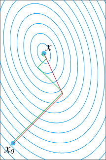
In mathematics, the conjugate gradient method is an algorithm for the numerical solution of particular systems of linear equations, namely those whose matrix is positive-definite. The conjugate gradient method is often implemented as an iterative algorithm, applicable to sparse systems that are too large to be handled by a direct implementation or other direct methods such as the Cholesky decomposition. Large sparse systems often arise when numerically solving partial differential equations or optimization problems.
The Kaczmarz method or Kaczmarz's algorithm is an iterative algorithm for solving linear equation systems . It was first discovered by the Polish mathematician Stefan Kaczmarz, and was rediscovered in the field of image reconstruction from projections by Richard Gordon, Robert Bender, and Gabor Herman in 1970, where it is called the Algebraic Reconstruction Technique (ART). ART includes the positivity constraint, making it nonlinear.
In mathematics, the generalized minimal residual method (GMRES) is an iterative method for the numerical solution of an indefinite nonsymmetric system of linear equations. The method approximates the solution by the vector in a Krylov subspace with minimal residual. The Arnoldi iteration is used to find this vector.
In the mathematical field of set theory, the proper forcing axiom (PFA) is a significant strengthening of Martin's axiom, where forcings with the countable chain condition (ccc) are replaced by proper forcings.
In computational chemistry, a constraint algorithm is a method for satisfying the Newtonian motion of a rigid body which consists of mass points. A restraint algorithm is used to ensure that the distance between mass points is maintained. The general steps involved are: (i) choose novel unconstrained coordinates, (ii) introduce explicit constraint forces, (iii) minimize constraint forces implicitly by the technique of Lagrange multipliers or projection methods.
The adjoint state method is a numerical method for efficiently computing the gradient of a function or operator in a numerical optimization problem. It has applications in geophysics, seismic imaging, photonics and more recently in neural networks.
Given a Hilbert space with a tensor product structure a product numerical range is defined as a numerical range with respect to the subset of product vectors. In some situations, especially in the context of quantum mechanics product numerical range is known as local numerical range
For computer science, in statistical learning theory, a representer theorem is any of several related results stating that a minimizer of a regularized empirical risk functional defined over a reproducing kernel Hilbert space can be represented as a finite linear combination of kernel products evaluated on the input points in the training set data.
Regularized least squares (RLS) is a family of methods for solving the least-squares problem while using regularization to further constrain the resulting solution.
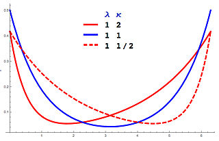
In probability theory and directional statistics, a wrapped asymmetric Laplace distribution is a wrapped probability distribution that results from the "wrapping" of the asymmetric Laplace distribution around the unit circle. For the symmetric case, the distribution becomes a wrapped Laplace distribution. The distribution of the ratio of two circular variates (Z) from two different wrapped exponential distributions will have a wrapped asymmetric Laplace distribution. These distributions find application in stochastic modelling of financial data.
Quantum optimization algorithms are quantum algorithms that are used to solve optimization problems. Mathematical optimization deals with finding the best solution to a problem from a set of possible solutions. Mostly, the optimization problem is formulated as a minimization problem, where one tries to minimize an error which depends on the solution: the optimal solution has the minimal error. Different optimization techniques are applied in various fields such as mechanics, economics and engineering, and as the complexity and amount of data involved rise, more efficient ways of solving optimization problems are needed. The power of quantum computing may allow problems which are not practically feasible on classical computers to be solved, or suggest a considerable speed up with respect to the best known classical algorithm.
Tau functions are an important ingredient in the modern theory of integrable systems, and have numerous applications in a variety of other domains. They were originally introduced by Ryogo Hirota in his direct method approach to soliton equations, based on expressing them in an equivalent bilinear form. The term Tau function, or -function, was first used systematically by Mikio Sato and his students in the specific context of the Kadomtsev–Petviashvili equation, and related integrable hierarchies. It is a central ingredient in the theory of solitons. Tau functions also appear as matrix model partition functions in the spectral theory of Random Matrices, and may also serve as generating functions, in the sense of combinatorics and enumerative geometry, especially in relation to moduli spaces of Riemann surfaces, and enumeration of branched coverings, or so-called Hurwitz numbers.


