Mathematical growth

Last updated November 20, 2023

Mathematical growth

Any process of non-random change that can be measured could be called mathematical growth (or decay). The change can be directly related to chronology (see Time series), or to any other input that can be arranged numerically. (As x "grows", what does y do?) There are many forms of this type of growth, including: linear, polynomial, and exponential, described by y = bx , y = ax^k , and y = ad^x , respectively, where x is the independent input variable, y the dependent output, and a, b, d and k are constants for each particular relationship. Of course, these mathematical models are idealized versions of the number patterns we see in the real world.

Linear growth

The growth rings of a tree. Each ring represents one year; the outside rings, near the bark, are the youngest. Tree.ring.arp.jpg — The growth rings of a tree. Each ring represents one year; the outside rings, near the bark, are the youngest.

Linear growth occurs whenever the change in the dependent variable y is directly proportional to the change in the independent variable x.^[1]^[2] (For example, when x is doubled, then y is doubled.) Because it is based on the addition of the same amount each time, linear growth is generally slow and steady.

Mathematically, linear growth is described by y = bx + c, where b is the amount added every time x increases by 1, and c is the value of y when x is 0. On a graph, b is the slope of the line, and c is the y-axis intercept. b is a rate, with units of y divided by the units of x.

A bank account with regular, uniform deposits and no interest exhibits linear growth. The diameter of a tree might display linear growth, year by year. Any process that can be modeled by the change in area of a parallelogram with one fixed side, or the change in volume of a cylinder or prism with a fixed base, is an example of linear growth. Linear growth can also be called additive or arithmetic growth.^[3]

Polynomial growth

Polynomial growth occurs when a parameter of the dependent variable changes linearly.^[2] This happens when the mathematical relationship involves a fixed exponent, often 2 (quadratic growth) or 3 (cubic growth).^[4] Although polynomial growth is based on multiplication, it is much slower than exponential growth, because of the fixed exponent on the slowly-changing base value.

Mathematically, equations for polynomial growth contain y = ax^k, where a is a compound rate (such as 32 ft/sec/sec) and k is a fixed exponent (greater than 1), both determined by the particular situation. Polynomial equations (also called power functions) may contain bx and/or c, whose characteristics are the same as in linear equations. (Technically, linear equations are a form of polynomial equation, with k = 1.)

Examples include the change in area of a triangle with a change in height, or the change in height of a falling object over time. The volume a triangular prism being filled in a direction parallel to the base, with respect to the height of the fill, is also an example of polynomial growth. (The rate of the filling itself is probably linear.)

Exponential growth

Exponential growth occurs when a parameter of the dependent variable changes geometrically (by multiplication).^[5] The mathematical relationship has the independent variable as the exponent on a rate of change. Because it is the exponent that varies, exponential growth is the fastest of all. Exponential growth is also called geometric growth.^[3]

Examples include a bank balance for an account with compounded interest and the number of ideally proliferating bacteria, not to mention the volume inside the horn of a brass musical instrument or Victrola, with respect to its height. Because few things in the real world grow exponentially forever, statisticians and others have defined the logistic growth curve,^[2] where the dependent variable grows exponentially at first, but then "inverts", or begins to level off in symmetrical fashion.^[6]

Interestingly, the well-known Fibonacci sequence is an example of exponential growth. Although the next value of the sequence can be found by adding the previous two, starting with 0 and 1 or 1 and 1, the general formula is exponential (see Binet's formula). The values in this particular sequence are found in many forms in nature, including the number of rabbits that spring from an original pair, the sizes of the chambers of a Nautilus shell, and the pattern of seeds of a sunflower.

Illustration of Vogel's model for n = 1 ... 500 SunflowerModel.svg — Illustration of Vogel's model for $n = 1 ... 500$

Determining type of growth

One can determine which type of growth a given set of data has by using regression modeling, which can be done with graphing calculators or computer software.^[2]^[7] Regression modeling uses statistical methods to find a "line of best fit" for the data. One generally has to try various possible models, such as power regression, exponential regression, etc., and choose the one with the highest correlation coefficient r.^[8]

If one knows the equation, or function, that describes some observed growth, one can use Big O analysis to characterize the type of growth. If the dependent variable is the number of elementary computer operations, the type of growth shown as the input amount changes can be found by analyzing the time complexity of the algorithm being used.

Related Research Articles

In mathematics, an equation is a mathematical formula that expresses the equality of two expressions, by connecting them with the equals sign =. The word equation and its cognates in other languages may have subtly different meanings; for example, in French an équation is defined as containing one or more variables, while in English, any well-formed formula consisting of two expressions related with an equals sign is an equation.

<span class="mw-page-title-main">Exponential function</span> Mathematical function, denoted exp(x) or e^x

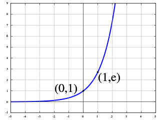
The exponential function is a mathematical function denoted by $or . Unless otherwise specified, the term generally refers to the positive-valued function of a real variable, although it can be extended to the complex numbers or generalized to other mathematical objects like matrices or Lie algebras. The exponential function originated from the notion of exponentiation, but modern definitions allow it to be rigorously extended to all real arguments, including irrational numbers. Its ubiquitous occurrence in pure and applied mathematics led mathematician Walter Rudin to opine that the exponential function is "the most important function in mathematics".$

In mathematics, a polynomial is an expression consisting of indeterminates and coefficients, that involves only the operations of addition, subtraction, multiplication, and positive-integer powers of variables. An example of a polynomial of a single indeterminate $x$ is $x 2 - 4 x + 7$ . An example with three indeterminates is $x 3 + 2 xyz 2 - yz + 1$ .

In mathematics, differential calculus is a subfield of calculus that studies the rates at which quantities change. It is one of the two traditional divisions of calculus, the other being integral calculus—the study of the area beneath a curve.

In mathematics, the term linear is used in two distinct senses for two different properties:

<span class="mw-page-title-main">Quadratic function</span> Polynomial function of degree two

In mathematics, a quadratic polynomial is a polynomial of degree two in one or more variables. A quadratic function is the polynomial function defined by a quadratic polynomial. Before the 20th century, the distinction was unclear between a polynomial and its associated polynomial function; so "quadratic polynomial" and "quadratic function" were almost synonymous. This is still the case in many elementary courses, where both terms are often abbreviated as "quadratic".

<span class="mw-page-title-main">Exponential growth</span> Growth of quantities at rate proportional to the current amount

Exponential growth is a process that increases quantity over time at an ever-increasing rate. It occurs when the instantaneous rate of change of a quantity with respect to time is proportional to the quantity itself. Described as a function, a quantity undergoing exponential growth is an exponential function of time, that is, the variable representing time is the exponent. Exponential growth is the inverse of logarithmic growth.

<span class="mw-page-title-main">Dependent and independent variables</span> Concept in mathematical modeling, statistical modeling and experimental sciences

Dependent and independent variables are variables in mathematical modeling, statistical modeling and experimental sciences. Dependent variables are studied under the supposition or demand that they depend, by some law or rule, on the values of other variables. Independent variables, in turn, are not seen as depending on any other variable in the scope of the experiment in question. In this sense, some common independent variables are time, space, density, mass, fluid flow rate, and previous values of some observed value of interest to predict future values.

Curve fitting is the process of constructing a curve, or mathematical function, that has the best fit to a series of data points, possibly subject to constraints. Curve fitting can involve either interpolation, where an exact fit to the data is required, or smoothing, in which a "smooth" function is constructed that approximately fits the data. A related topic is regression analysis, which focuses more on questions of statistical inference such as how much uncertainty is present in a curve that is fit to data observed with random errors. Fitted curves can be used as an aid for data visualization, to infer values of a function where no data are available, and to summarize the relationships among two or more variables. Extrapolation refers to the use of a fitted curve beyond the range of the observed data, and is subject to a degree of uncertainty since it may reflect the method used to construct the curve as much as it reflects the observed data.

In mathematics, an expression is in closed form if it is formed with constants, variables and a finite set of basic functions connected by arithmetic operations and function composition. Commonly, the allowed functions are nth root, exponential function, logarithm, and trigonometric functions. However, the set of basic functions depends on the context.

In statistics, a generalized linear model (GLM) is a flexible generalization of ordinary linear regression. The GLM generalizes linear regression by allowing the linear model to be related to the response variable via a link function and by allowing the magnitude of the variance of each measurement to be a function of its predicted value.

In statistical modeling, regression analysis is a set of statistical processes for estimating the relationships between a dependent variable and one or more independent variables. The most common form of regression analysis is linear regression, in which one finds the line that most closely fits the data according to a specific mathematical criterion. For example, the method of ordinary least squares computes the unique line that minimizes the sum of squared differences between the true data and that line. For specific mathematical reasons, this allows the researcher to estimate the conditional expectation of the dependent variable when the independent variables take on a given set of values. Less common forms of regression use slightly different procedures to estimate alternative location parameters or estimate the conditional expectation across a broader collection of non-linear models.

In statistics, nonlinear regression is a form of regression analysis in which observational data are modeled by a function which is a nonlinear combination of the model parameters and depends on one or more independent variables. The data are fitted by a method of successive approximations.

In mathematics, a variable is a symbol that represents a mathematical object. A variable may represent a number, a vector, a matrix, a function, the argument of a function, a set, or an element of a set.

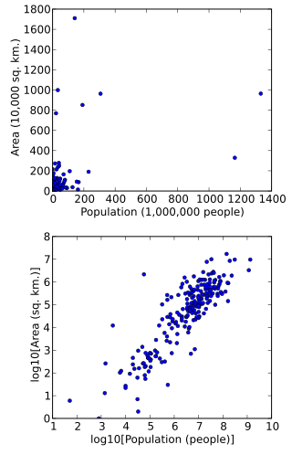
In statistics, data transformation is the application of a deterministic mathematical function to each point in a data set—that is, each data point z_i is replaced with the transformed value y_i = f(z_i), where f is a function. Transforms are usually applied so that the data appear to more closely meet the assumptions of a statistical inference procedure that is to be applied, or to improve the interpretability or appearance of graphs.

In statistics and econometrics, a distributed lag model is a model for time series data in which a regression equation is used to predict current values of a dependent variable based on both the current values of an explanatory variable and the lagged values of this explanatory variable.

In statistics, polynomial regression is a form of regression analysis in which the relationship between the independent variable x and the dependent variable y is modelled as an nth degree polynomial in x. Polynomial regression fits a nonlinear relationship between the value of x and the corresponding conditional mean of y, denoted E(y |x). Although polynomial regression fits a nonlinear model to the data, as a statistical estimation problem it is linear, in the sense that the regression function E(y | x) is linear in the unknown parameters that are estimated from the data. For this reason, polynomial regression is considered to be a special case of multiple linear regression.

In statistics and in machine learning, a linear predictor function is a linear function of a set of coefficients and explanatory variables, whose value is used to predict the outcome of a dependent variable. This sort of function usually comes in linear regression, where the coefficients are called regression coefficients. However, they also occur in various types of linear classifiers, as well as in various other models, such as principal component analysis and factor analysis. In many of these models, the coefficients are referred to as "weights".

<span class="mw-page-title-main">Linear function (calculus)</span> Polynomial function of degree at most one

In calculus and related areas of mathematics, a linear function from the real numbers to the real numbers is a function whose graph is a non-vertical line in the plane. The characteristic property of linear functions is that when the input variable is changed, the change in the output is proportional to the change in the input.

In statistics, linear regression is a linear approach for modelling the relationship between a scalar response and one or more explanatory variables. The case of one explanatory variable is called simple linear regression; for more than one, the process is called multiple linear regression. This term is distinct from multivariate linear regression, where multiple correlated dependent variables are predicted, rather than a single scalar variable.

References

↑ "Section 4.1: Linear Growth" (PDF). Coconino Community College, Mathematics Department.
1 2 3 4 Gilchrist, Warren (1984). Statistical Modelling. Chichester, UK: John Wiley & Sons. p. 61 ff.(a); 64(b); 71(c); 61(d).
1 2 Foster, Alan G. (1995). Merrill Algebra 2 with Trigonometry. New York: Glencoe/McGraw-Hill. p. 596(a); 608(b).
↑ "How do you explain cubic growth of a function". stackexchange.com.
↑ Serway, Raymond A. & Jerry S. Faughn (1992). College Physics, Third Edition. Fort Worth: Harcourt Brace. p. 690.
↑ Griffin, John I. (1962). Statistics-Methods and Applications. New York: Holt, Rinehart and Winston. p. 335.
↑ TI-83 Plus Graphing Calculator Guidebook; Section 12-22, Regression Model Features. Dallas: Texas Instruments Inc. 1999.
↑ Yates, Daniel S. (2008). The Practice of Statistics. New York: W.H. Freeman & Co. p. 209 ff.

Sources

Foster, Alan G. et al, "Merrill - Algebra 2 with Trigonometry", Glencoe/McGraw-Hill, New York, 1995.
Gilchrist, Warren, "Statistical Modelling", John Wiley & Sons, Chichester, UK, 1984.
Yates, Daniel S., et al, "The Practice of Statistics, Third Edition", W.H. Freeman & Co., New York, 2008; Ch. 4: Relationships Between Two Variables.

External links

https://www.nytimes.com/2019/03/04/opinion/exponential-language-math.html?searchResultPosition=9

This page is based on this Wikipedia article
Text is available under the CC BY-SA 4.0 license; additional terms may apply.
Images, videos and audio are available under their respective licenses.

[1] "Section 4.1: Linear Growth" (PDF). Coconino Community College, Mathematics Department.

[Gilchrist-1984-2] 1 2 3 4 Gilchrist, Warren (1984). Statistical Modelling. Chichester, UK: John Wiley & Sons. p. 61 ff.(a); 64(b); 71(c); 61(d).

[Foster-1995-3] 1 2 Foster, Alan G. (1995). Merrill Algebra 2 with Trigonometry. New York: Glencoe/McGraw-Hill. p. 596(a); 608(b).

[4] "How do you explain cubic growth of a function". stackexchange.com.

[Serway-1992-5] Serway, Raymond A. & Jerry S. Faughn (1992). College Physics, Third Edition. Fort Worth: Harcourt Brace. p. 690.

[Griffin-1962-6] Griffin, John I. (1962). Statistics-Methods and Applications. New York: Holt, Rinehart and Winston. p. 335.

[7] TI-83 Plus Graphing Calculator Guidebook; Section 12-22, Regression Model Features. Dallas: Texas Instruments Inc. 1999.

[Yates-2008-8] Yates, Daniel S. (2008). The Practice of Statistics. New York: W.H. Freeman & Co. p. 209 ff.

[1]

[2]

[3]

[4]

[5]

[6]

[7]

[8]

..Count	..Linear	...Fibonacci	Polynomial	Exponential
x (or n)	y_x = 2x	y_x = y_x−1+y_x−2	y_x = x²	y_x = 2^x
0	0	0	0	1
1	2	1	1	2
2	4	1	4	4
3	6	2	9	8
4	8	3	16	16
5	10	5	25	32
6	12	8	36	64
7	14	13	49	128
8	16	21	64	256
9	18	34	81	512
10	20	55	100	1024
11	22	89	121	2048
12	24	144	144	4096
13	26	233	169	8192
14	28	377	196	16384
15	30	610	225	32768

Mathematical growth