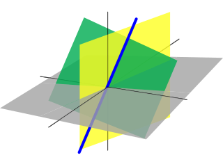
In mathematics, Gaussian elimination, also known as row reduction, is an algorithm for solving systems of linear equations. It consists of a sequence of operations performed on the corresponding matrix of coefficients. This method can also be used to compute the rank of a matrix, the determinant of a square matrix, and the inverse of an invertible matrix. The method is named after Carl Friedrich Gauss (1777–1855). To perform row reduction on a matrix, one uses a sequence of elementary row operations to modify the matrix until the lower left-hand corner of the matrix is filled with zeros, as much as possible. There are three types of elementary row operations:

Linear algebra is the branch of mathematics concerning linear equations such as:
In linear algebra, the rank of a matrix A is the dimension of the vector space generated by its columns. This corresponds to the maximal number of linearly independent columns of A. This, in turn, is identical to the dimension of the vector space spanned by its rows. Rank is thus a measure of the "nondegenerateness" of the system of linear equations and linear transformation encoded by A. There are multiple equivalent definitions of rank. A matrix's rank is one of its most fundamental characteristics.

In mathematics, and more specifically in linear algebra, a linear subspace or vector subspace is a vector space that is a subset of some larger vector space. A linear subspace is usually simply called a subspace when the context serves to distinguish it from other types of subspaces.

In mathematics, a system of linear equations is a collection of one or more linear equations involving the same variables.
In linear algebra, an n-by-n square matrix A is called invertible, if there exists an n-by-n square matrix B such that
In linear algebra, a matrix may always be put into row or column echelon form, by applying elementary row operations, or elementary column operations, respectively; in particular, this can be done using the Gaussian elimination method.

In numerical analysis and scientific computing, a sparse matrix or sparse array is a matrix in which most of the elements are zero. There is no strict definition regarding the proportion of zero-value elements for a matrix to qualify as sparse but a common criterion is that the number of non-zero elements is roughly equal to the number of rows or columns. By contrast, if most of the elements are non-zero, the matrix is considered dense. The number of zero-valued elements divided by the total number of elements is sometimes referred to as the sparsity of the matrix.
In mathematical optimization, Dantzig's simplex algorithm is a popular algorithm for linear programming.
In numerical analysis, the minimum degree algorithm is an algorithm used to permute the rows and columns of a symmetric sparse matrix before applying the Cholesky decomposition, to reduce the number of non-zeros in the Cholesky factor. This results in reduced storage requirements and means that the Cholesky factor can be applied with fewer arithmetic operations.
In mathematics, the kernel of a linear map, also known as the null space or nullspace, is the linear subspace of the domain of the map which is mapped to the zero vector. That is, given a linear map L : V → W between two vector spaces V and W, the kernel of L is the vector space of all elements v of V such that L(v) = 0, where 0 denotes the zero vector in W, or more symbolically:
In mathematics, particularly matrix theory, a band matrix or banded matrix is a sparse matrix whose non-zero entries are confined to a diagonal band, comprising the main diagonal and zero or more diagonals on either side.
In numerical linear algebra, the Jacobi eigenvalue algorithm is an iterative method for the calculation of the eigenvalues and eigenvectors of a real symmetric matrix. It is named after Carl Gustav Jacob Jacobi, who first proposed the method in 1846, but only became widely used in the 1950s with the advent of computers.
In numerical analysis and linear algebra, lower–upper (LU) decomposition or factorization factors a matrix as the product of a lower triangular matrix and an upper triangular matrix. The product sometimes includes a permutation matrix as well. LU decomposition can be viewed as the matrix form of Gaussian elimination. Computers usually solve square systems of linear equations using LU decomposition, and it is also a key step when inverting a matrix or computing the determinant of a matrix. The LU decomposition was introduced by the Polish astronomer Tadeusz Banachiewicz in 1938. To quote: "It appears that Gauss and Doolittle applied the method [of elimination] only to symmetric equations. More recent authors, for example, Aitken, Banachiewicz, Dwyer, and Crout … have emphasized the use of the method, or variations of it, in connection with non-symmetric problems … Banachiewicz … saw the point … that the basic problem is really one of matrix factorization, or “decomposition” as he called it." It's also referred to as LR decomposition.
Numerical linear algebra, sometimes called applied linear algebra, is the study of how matrix operations can be used to create computer algorithms which efficiently and accurately provide approximate answers to questions in continuous mathematics. It is a subfield of numerical analysis, and a type of linear algebra. Computers use floating-point arithmetic and cannot exactly represent irrational data, so when a computer algorithm is applied to a matrix of data, it can sometimes increase the difference between a number stored in the computer and the true number that it is an approximation of. Numerical linear algebra uses properties of vectors and matrices to develop computer algorithms that minimize the error introduced by the computer, and is also concerned with ensuring that the algorithm is as efficient as possible.
In linear algebra, the Hermite normal form is an analogue of reduced echelon form for matrices over the integers Z. Just as reduced echelon form can be used to solve problems about the solution to the linear system Ax=b where x is in Rn, the Hermite normal form can solve problems about the solution to the linear system Ax=b where this time x is restricted to have integer coordinates only. Other applications of the Hermite normal form include integer programming, cryptography, and abstract algebra.
In mathematics, a system of equations is considered overdetermined if there are more equations than unknowns. An overdetermined system is almost always inconsistent when constructed with random coefficients. However, an overdetermined system will have solutions in some cases, for example if some equation occurs several times in the system, or if some equations are linear combinations of the others.
In mathematics, the Bareiss algorithm, named after Erwin Bareiss, is an algorithm to calculate the determinant or the echelon form of a matrix with integer entries using only integer arithmetic; any divisions that are performed are guaranteed to be exact. The method can also be used to compute the determinant of matrices with (approximated) real entries, avoiding the introduction of any round-off errors beyond those already present in the input.

In mathematics, a matrix is a rectangular array or table of numbers, symbols, or expressions, arranged in rows and columns, which is used to represent a mathematical object or a property of such an object.


