Point distribution model

Last updated January 12, 2022

The point distribution model is a model for representing the mean geometry of a shape and some statistical modes of geometric variation inferred from a training set of shapes.

Background

The point distribution model concept has been developed by Cootes,^[1] Taylor et al.^[2] and became a standard in computer vision for the statistical study of shape ^[3] and for segmentation of medical images ^[2] where shape priors really help interpretation of noisy and low-contrasted pixels/voxels. The latter point leads to active shape models (ASM) and active appearance models (AAM).

Point distribution models rely on landmark points. A landmark is an annotating point posed by an anatomist onto a given locus for every shape instance across the training set population. For instance, the same landmark will designate the tip of the index finger in a training set of 2D hands outlines. Principal component analysis (PCA), for instance, is a relevant tool for studying correlations of movement between groups of landmarks among the training set population. Typically, it might detect that all the landmarks located along the same finger move exactly together across the training set examples showing different finger spacing for a flat-posed hands collection.

Details

First, a set of training images are manually landmarked with enough corresponding landmarks to sufficiently approximate the geometry of the original shapes. These landmarks are aligned using the generalized procrustes analysis, which minimizes the least squared error between the points.

$k$ aligned landmarks in two dimensions are given as

\mathbf {X} =(x_{1},y_{1},\ldots ,x_{k},y_{k})

.

It's important to note that each landmark $i\in \lbrace 1,\ldots k\rbrace$ should represent the same anatomical location. For example, landmark #3, $(x_{3},y_{3})$ might represent the tip of the ring finger across all training images.

Now the shape outlines are reduced to sequences of $k$ landmarks, so that a given training shape is defined as the vector $\mathbf {X} \in \mathbb {R} ^{2k}$ . Assuming the scattering is gaussian in this space, PCA is used to compute normalized eigenvectors and eigenvalues of the covariance matrix across all training shapes. The matrix of the top $d$ eigenvectors is given as $\mathbf {P} \in \mathbb {R} ^{2k\times d}$ , and each eigenvector describes a principal mode of variation along the set.

Finally, a linear combination of the eigenvectors is used to define a new shape $\mathbf {X} '$ , mathematically defined as:

\mathbf {X} '={\overline {\mathbf {X} }}+\mathbf {P} \mathbf {b}

where ${\overline {\mathbf {X} }}$ is defined as the mean shape across all training images, and $\mathbf {b}$ is a vector of scaling values for each principal component. Therefore, by modifying the variable $\mathbf {b}$ an infinite number of shapes can be defined. To ensure that the new shapes are all within the variation seen in the training set, it is common to only allow each element of $\mathbf {b}$ to be within $\pm$ 3 standard deviations, where the standard deviation of a given principal component is defined as the square root of its corresponding eigenvalue.

PDM's can be extended to any arbitrary number of dimensions, but are typically used in 2D image and 3D volume applications (where each landmark point is $\mathbb {R} ^{2}$ or $\mathbb {R} ^{3}$ ).

Discussion

An eigenvector, interpreted in euclidean space, can be seen as a sequence of $k$ euclidean vectors associated to corresponding landmark and designating a compound move for the whole shape. Global nonlinear variation is usually well handled provided nonlinear variation is kept to a reasonable level. Typically, a twisting nematode worm is used as an example in the teaching of kernel PCA-based methods.

Due to the PCA properties: eigenvectors are mutually orthogonal, form a basis of the training set cloud in the shape space, and cross at the 0 in this space, which represents the mean shape. Also, PCA is a traditional way of fitting a closed ellipsoid to a Gaussian cloud of points (whatever their dimension): this suggests the concept of bounded variation.

The idea behind PDMs is that eigenvectors can be linearly combined to create an infinity of new shape instances that will 'look like' the one in the training set. The coefficients are bounded alike the values of the corresponding eigenvalues, so as to ensure the generated 2n/3n-dimensional dot will remain into the hyper-ellipsoidal allowed domain—allowable shape domain (ASD).^[2]

Related Research Articles

In mathematics, the discrete Fourier transform (DFT) converts a finite sequence of equally-spaced samples of a function into a same-length sequence of equally-spaced samples of the discrete-time Fourier transform (DTFT), which is a complex-valued function of frequency. The interval at which the DTFT is sampled is the reciprocal of the duration of the input sequence. An inverse DFT is a Fourier series, using the DTFT samples as coefficients of complex sinusoids at the corresponding DTFT frequencies. It has the same sample-values as the original input sequence. The DFT is therefore said to be a frequency domain representation of the original input sequence. If the original sequence spans all the non-zero values of a function, its DTFT is continuous, and the DFT provides discrete samples of one cycle. If the original sequence is one cycle of a periodic function, the DFT provides all the non-zero values of one DTFT cycle.

In mathematics, a symmetric matrix $with real entries is positive-definite if the real number is positive for every nonzero real column vector where is the transpose of . More generally, a Hermitian matrix is positive-definite if the real number is positive for every nonzero complex column vector where denotes the conjugate transpose of$

Principal component analysis Conversion of observations of possibly-correlated variables into values of fewer, uncorrelated variables

The principal components of a collection of points in a real coordinate space are a sequence of $unit vectors, where the -th vector is the direction of a line that best fits the data while being orthogonal to the first vectors. Here, a best-fitting line is defined as one that minimizes the average squared distance from the points to the line. These directions constitute an orthonormal basis in which different individual dimensions of the data are linearly uncorrelated. Principal component analysis (PCA) is the process of computing the principal components and using them to perform a change of basis on the data, sometimes using only the first few principal components and ignoring the rest.$

Singular value decomposition Matrix decomposition

In linear algebra, the singular value decomposition (SVD) is a factorization of a real or complex matrix. It generalizes the eigendecomposition of a square normal matrix with an orthonormal eigenbasis to any $matrix. It is related to the polar decomposition.$

In mathematics, a self-adjoint operator on an infinite-dimensional complex vector space V with inner product $is a linear map A that is its own adjoint. If V is finite-dimensional with a given orthonormal basis, this is equivalent to the condition that the matrix of A is a Hermitian matrix, i.e., equal to its conjugate transpose A * . By the finite-dimensional spectral theorem, V has an orthonormal basis such that the matrix of A relative to this basis is a diagonal matrix with entries in the real numbers. In this article, we consider generalizations of this concept to operators on Hilbert spaces of arbitrary dimension.$

In linear algebra, a square matrix $is called diagonalizable or non-defective if it is similar to a diagonal matrix, i.e., if there exists an invertible matrix and a diagonal matrix such that, or equivalently . For a finite-dimensional vector space, a linear map is called diagonalizable if there exists an ordered basis of consisting of eigenvectors of . These definitions are equivalent: if has a matrix representation as above, then the column vectors of form a basis consisting of eigenvectors of, and the diagonal entries of are the corresponding eigenvalues of; with respect to this eigenvector basis, is represented by . Diagonalization is the process of finding the above and .$

In physics, an operator is a function over a space of physical states onto another space of physical states. The simplest example of the utility of operators is the study of symmetry. Because of this, they are very useful tools in classical mechanics. Operators are even more important in quantum mechanics, where they form an intrinsic part of the formulation of the theory.

High-dimensional data, meaning data that requires more than two or three dimensions to represent, can be difficult to interpret. One approach to simplification is to assume that the data of interest lies within lower-dimensional space. If the data of interest is of low enough dimension, the data can be visualised in the low-dimensional space.

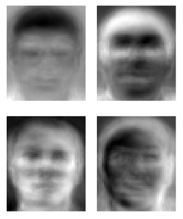
An eigenface is the name given to a set of eigenvectors when used in the computer vision problem of human face recognition. The approach of using eigenfaces for recognition was developed by Sirovich and Kirby and used by Matthew Turk and Alex Pentland in face classification. The eigenvectors are derived from the covariance matrix of the probability distribution over the high-dimensional vector space of face images. The eigenfaces themselves form a basis set of all images used to construct the covariance matrix. This produces dimension reduction by allowing the smaller set of basis images to represent the original training images. Classification can be achieved by comparing how faces are represented by the basis set.

In mathematics, a canonical basis is a basis of an algebraic structure that is canonical in a sense that depends on the precise context:

The Rayleigh–Ritz method is a direct numerical method of approximating eigenvalue, originated in the context of solving physical boundary value problems and named after Lord Rayleigh and Walther Ritz.

In linear algebra, an eigenvector or characteristic vector of a linear transformation is a nonzero vector that changes at most by a scalar factor when that linear transformation is applied to it. The corresponding eigenvalue, often denoted by $, is the factor by which the eigenvector is scaled.$

In quantum mechanics, the position operator is the operator that corresponds to the position observable of a particle.

In the field of multivariate statistics, kernel principal component analysis is an extension of principal component analysis (PCA) using techniques of kernel methods. Using a kernel, the originally linear operations of PCA are performed in a reproducing kernel Hilbert space.

In functional analysis, the concept of a compact operator on Hilbert space is an extension of the concept of a matrix acting on a finite-dimensional vector space; in Hilbert space, compact operators are precisely the closure of finite-rank operators in the topology induced by the operator norm. As such, results from matrix theory can sometimes be extended to compact operators using similar arguments. By contrast, the study of general operators on infinite-dimensional spaces often requires a genuinely different approach.

In linear algebra, eigendecomposition is the factorization of a matrix into a canonical form, whereby the matrix is represented in terms of its eigenvalues and eigenvectors. Only diagonalizable matrices can be factorized in this way. When the matrix being factorized is a normal or real symmetric matrix, the decomposition is called "spectral decomposition", derived from the spectral theorem.

In multivariate statistics, spectral clustering techniques make use of the spectrum (eigenvalues) of the similarity matrix of the data to perform dimensionality reduction before clustering in fewer dimensions. The similarity matrix is provided as an input and consists of a quantitative assessment of the relative similarity of each pair of points in the dataset.

In statistics, principal component regression (PCR) is a regression analysis technique that is based on principal component analysis (PCA). More specifically, PCR is used for estimating the unknown regression coefficients in a standard linear regression model.

In mathematics, and especially affine differential geometry, the affine focal set of a smooth submanifold M embedded in a smooth manifold N is the caustic generated by the affine normal lines. It can be realised as the bifurcation set of a certain family of functions. The bifurcation set is the set of parameter values of the family which yield functions with degenerate singularities. This is not the same as the bifurcation diagram in dynamical systems.

In mathematics, particularly in linear algebra and applications, matrix analysis is the study of matrices and their algebraic properties. Some particular topics out of many include; operations defined on matrices, functions of matrices, and the eigenvalues of matrices.

References

↑ T. F. Cootes (May 2004), Statistical models of appearance for computer vision (PDF)
1 2 3 D.H. Cooper; T.F. Cootes; C.J. Taylor; J. Graham (1995), "Active shape models—their training and application", Computer Vision and Image Understanding (61): 38–59
↑ Rhodri H. Davies and Carole J. Twining and P. Daniel Allen and Tim F. Cootes and Chris J. Taylor (2003). Shape discrimination in the Hippocampus using an MDL Model. IMPI. Archived from the original on 2008-10-08. Retrieved 2007-07-27.

External links

Flexible Models for Computer Vision, Tim Cootes, Manchester University.
A practical introduction to PDM and ASMs.

This page is based on this Wikipedia article
Text is available under the CC BY-SA 4.0 license; additional terms may apply.
Images, videos and audio are available under their respective licenses.

[1] T. F. Cootes (May 2004), Statistical models of appearance for computer vision (PDF)

[taylor-2] 1 2 3 D.H. Cooper; T.F. Cootes; C.J. Taylor; J. Graham (1995), "Active shape models—their training and application", Computer Vision and Image Understanding (61): 38–59

[3] Rhodri H. Davies and Carole J. Twining and P. Daniel Allen and Tim F. Cootes and Chris J. Taylor (2003). Shape discrimination in the Hippocampus using an MDL Model. IMPI. Archived from the original on 2008-10-08. Retrieved 2007-07-27.

[1]

[2]

[3]