In vector calculus, divergence is a vector operator that operates on a vector field, producing a scalar field giving the quantity of the vector field's source at each point. More technically, the divergence represents the volume density of the outward flux of a vector field from an infinitesimal volume around a given point.
The Cauchy–Schwarz inequality is an upper bound on the inner product between two vectors in an inner product space in terms of the product of the vector norms. It is considered one of the most important and widely used inequalities in mathematics.

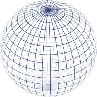
In mathematics, an n-sphere or hypersphere is an -dimensional generalization of the -dimensional circle and -dimensional sphere to any non-negative integer . The -sphere is the setting for -dimensional spherical geometry.
In machine learning, support vector machines are supervised max-margin models with associated learning algorithms that analyze data for classification and regression analysis. Developed at AT&T Bell Laboratories by Vladimir Vapnik with colleagues SVMs are one of the most studied models, being based on statistical learning frameworks of VC theory proposed by Vapnik and Chervonenkis (1974).
In the mathematical field of differential geometry, a metric tensor is an additional structure on a manifold M that allows defining distances and angles, just as the inner product on a Euclidean space allows defining distances and angles there. More precisely, a metric tensor at a point p of M is a bilinear form defined on the tangent space at p, and a metric field on M consists of a metric tensor at each point p of M that varies smoothly with p.

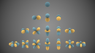
In mathematics and physical science, spherical harmonics are special functions defined on the surface of a sphere. They are often employed in solving partial differential equations in many scientific fields. The table of spherical harmonics contains a list of common spherical harmonics.
In mathematics, a linear form is a linear map from a vector space to its field of scalars.
In vector calculus, Green's theorem relates a line integral around a simple closed curve C to a double integral over the plane region D bounded by C. It is the two-dimensional special case of Stokes' theorem. In one dimension, it is equivalent to the fundamental theorem of calculus. In three dimensions, it is equivalent to the divergence theorem.

In mathematics, a Green's function is the impulse response of an inhomogeneous linear differential operator defined on a domain with specified initial conditions or boundary conditions.
In mathematics, the covariant derivative is a way of specifying a derivative along tangent vectors of a manifold. Alternatively, the covariant derivative is a way of introducing and working with a connection on a manifold by means of a differential operator, to be contrasted with the approach given by a principal connection on the frame bundle – see affine connection. In the special case of a manifold isometrically embedded into a higher-dimensional Euclidean space, the covariant derivative can be viewed as the orthogonal projection of the Euclidean directional derivative onto the manifold's tangent space. In this case the Euclidean derivative is broken into two parts, the extrinsic normal component and the intrinsic covariant derivative component.

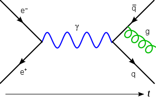
In quantum field theory, the Lehmann–Symanzik–Zimmermann (LSZ) reduction formula is a method to calculate S-matrix elements from the time-ordered correlation functions of a quantum field theory. It is a step of the path that starts from the Lagrangian of some quantum field theory and leads to prediction of measurable quantities. It is named after the three German physicists Harry Lehmann, Kurt Symanzik and Wolfhart Zimmermann.
In machine learning, kernel machines are a class of algorithms for pattern analysis, whose best known member is the support-vector machine (SVM). These methods involve using linear classifiers to solve nonlinear problems. The general task of pattern analysis is to find and study general types of relations in datasets. For many algorithms that solve these tasks, the data in raw representation have to be explicitly transformed into feature vector representations via a user-specified feature map: in contrast, kernel methods require only a user-specified kernel, i.e., a similarity function over all pairs of data points computed using inner products. The feature map in kernel machines is infinite dimensional but only requires a finite dimensional matrix from user-input according to the Representer theorem. Kernel machines are slow to compute for datasets larger than a couple of thousand examples without parallel processing.
In applied mathematics, polyharmonic splines are used for function approximation and data interpolation. They are very useful for interpolating and fitting scattered data in many dimensions. Special cases include thin plate splines and natural cubic splines in one dimension.
In physics and mathematics, the solid harmonics are solutions of the Laplace equation in spherical polar coordinates, assumed to be (smooth) functions . There are two kinds: the regular solid harmonics, which are well-defined at the origin and the irregular solid harmonics, which are singular at the origin. Both sets of functions play an important role in potential theory, and are obtained by rescaling spherical harmonics appropriately:
In mathematics, vector spherical harmonics (VSH) are an extension of the scalar spherical harmonics for use with vector fields. The components of the VSH are complex-valued functions expressed in the spherical coordinate basis vectors.
In the finite element method for the numerical solution of elliptic partial differential equations, the stiffness matrix is a matrix that represents the system of linear equations that must be solved in order to ascertain an approximate solution to the differential equation.
Least-squares support-vector machines (LS-SVM) for statistics and in statistical modeling, are least-squares versions of support-vector machines (SVM), which are a set of related supervised learning methods that analyze data and recognize patterns, and which are used for classification and regression analysis. In this version one finds the solution by solving a set of linear equations instead of a convex quadratic programming (QP) problem for classical SVMs. Least-squares SVM classifiers were proposed by Johan Suykens and Joos Vandewalle. LS-SVMs are a class of kernel-based learning methods.
Within bayesian statistics for machine learning, kernel methods arise from the assumption of an inner product space or similarity structure on inputs. For some such methods, such as support vector machines (SVMs), the original formulation and its regularization were not Bayesian in nature. It is helpful to understand them from a Bayesian perspective. Because the kernels are not necessarily positive semidefinite, the underlying structure may not be inner product spaces, but instead more general reproducing kernel Hilbert spaces. In Bayesian probability kernel methods are a key component of Gaussian processes, where the kernel function is known as the covariance function. Kernel methods have traditionally been used in supervised learning problems where the input space is usually a space of vectors while the output space is a space of scalars. More recently these methods have been extended to problems that deal with multiple outputs such as in multi-task learning.
In machine learning, the radial basis function kernel, or RBF kernel, is a popular kernel function used in various kernelized learning algorithms. In particular, it is commonly used in support vector machine classification.
In machine learning, the kernel embedding of distributions comprises a class of nonparametric methods in which a probability distribution is represented as an element of a reproducing kernel Hilbert space (RKHS). A generalization of the individual data-point feature mapping done in classical kernel methods, the embedding of distributions into infinite-dimensional feature spaces can preserve all of the statistical features of arbitrary distributions, while allowing one to compare and manipulate distributions using Hilbert space operations such as inner products, distances, projections, linear transformations, and spectral analysis. This learning framework is very general and can be applied to distributions over any space on which a sensible kernel function may be defined. For example, various kernels have been proposed for learning from data which are: vectors in , discrete classes/categories, strings, graphs/networks, images, time series, manifolds, dynamical systems, and other structured objects. The theory behind kernel embeddings of distributions has been primarily developed by Alex Smola, Le Song , Arthur Gretton, and Bernhard Schölkopf. A review of recent works on kernel embedding of distributions can be found in.


