In probability theory and statistics, kurtosis is a measure of the "tailedness" of the probability distribution of a real-valued random variable. Like skewness, kurtosis describes a particular aspect of a probability distribution. There are different ways to quantify kurtosis for a theoretical distribution, and there are corresponding ways of estimating it using a sample from a population. Different measures of kurtosis may have different interpretations.

In statistics and probability theory, the median is the value separating the higher half from the lower half of a data sample, a population, or a probability distribution. For a data set, it may be thought of as "the middle" value. The basic feature of the median in describing data compared to the mean is that it is not skewed by a small proportion of extremely large or small values, and therefore provides a better representation of the center. Median income, for example, may be a better way to describe center of the income distribution because increases in the largest incomes alone have no effect on median. For this reason, the median is of central importance in robust statistics.

In statistics, the standard deviation is a measure of the amount of variation or dispersion of a set of values. A low standard deviation indicates that the values tend to be close to the mean of the set, while a high standard deviation indicates that the values are spread out over a wider range.

In probability theory and statistics, skewness is a measure of the asymmetry of the probability distribution of a real-valued random variable about its mean. The skewness value can be positive, zero, negative, or undefined.

In statistics, an outlier is a data point that differs significantly from other observations. An outlier may be due to a variability in the measurement, an indication of novel data, or it may be the result of experimental error; the latter are sometimes excluded from the data set. An outlier can be an indication of exciting possibility, but can also cause serious problems in statistical analyses.
In statistics, the mean squared error (MSE) or mean squared deviation (MSD) of an estimator measures the average of the squares of the errors—that is, the average squared difference between the estimated values and the actual value. MSE is a risk function, corresponding to the expected value of the squared error loss. The fact that MSE is almost always strictly positive is because of randomness or because the estimator does not account for information that could produce a more accurate estimate. In machine learning, specifically empirical risk minimization, MSE may refer to the empirical risk, as an estimate of the true MSE.
In statistics and optimization, errors and residuals are two closely related and easily confused measures of the deviation of an observed value of an element of a statistical sample from its "true value". The error of an observation is the deviation of the observed value from the true value of a quantity of interest. The residual is the difference between the observed value and the estimated value of the quantity of interest. The distinction is most important in regression analysis, where the concepts are sometimes called the regression errors and regression residuals and where they lead to the concept of studentized residuals. In econometrics, "errors" are also called disturbances.
In statistical inference, specifically predictive inference, a prediction interval is an estimate of an interval in which a future observation will fall, with a certain probability, given what has already been observed. Prediction intervals are often used in regression analysis.
In statistics a minimum-variance unbiased estimator (MVUE) or uniformly minimum-variance unbiased estimator (UMVUE) is an unbiased estimator that has lower variance than any other unbiased estimator for all possible values of the parameter.
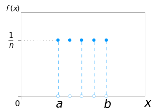
In probability theory and statistics, the discrete uniform distribution is a symmetric probability distribution wherein a finite number of values are equally likely to be observed; every one of n values has equal probability 1/n. Another way of saying "discrete uniform distribution" would be "a known, finite number of outcomes equally likely to happen".

In probability theory and statistics, the continuous uniform distributions or rectangular distributions are a family of symmetric probability distributions. Such a distribution describes an experiment where there is an arbitrary outcome that lies between certain bounds. The bounds are defined by the parameters, and which are the minimum and maximum values. The interval can either be closed or open. Therefore, the distribution is often abbreviated where stands for uniform distribution. The difference between the bounds defines the interval length; all intervals of the same length on the distribution's support are equally probable. It is the maximum entropy probability distribution for a random variable under no constraint other than that it is contained in the distribution's support.
This glossary of statistics and probability is a list of definitions of terms and concepts used in the mathematical sciences of statistics and probability, their sub-disciplines, and related fields. For additional related terms, see Glossary of mathematics and Glossary of experimental design.
In statistics, the mid-range or mid-extreme is a measure of central tendency of a sample defined as the arithmetic mean of the maximum and minimum values of the data set:
Robust statistics are statistics with good performance for data drawn from a wide range of probability distributions, especially for distributions that are not normal. Robust statistical methods have been developed for many common problems, such as estimating location, scale, and regression parameters. One motivation is to produce statistical methods that are not unduly affected by outliers. Another motivation is to provide methods with good performance when there are small departures from a parametric distribution. For example, robust methods work well for mixtures of two normal distributions with different standard deviations; under this model, non-robust methods like a t-test work poorly.
In statistics, the frequency of an event is the number of times the observation has occurred/recorded in an experiment or study. These frequencies are often depicted graphically or in tabular form.
In statistics, a pivotal quantity or pivot is a function of observations and unobservable parameters such that the function's probability distribution does not depend on the unknown parameters. A pivot quantity need not be a statistic—the function and its value can depend on the parameters of the model, but its distribution must not. If it is a statistic, then it is known as an ancillary statistic.
In statistics, the t-statistic is the ratio of the departure of the estimated value of a parameter from its hypothesized value to its standard error. It is used in hypothesis testing via Student's t-test. The t-statistic is used in a t-test to determine whether to support or reject the null hypothesis. It is very similar to the z-score but with the difference that t-statistic is used when the sample size is small or the population standard deviation is unknown. For example, the t-statistic is used in estimating the population mean from a sampling distribution of sample means if the population standard deviation is unknown. It is also used along with p-value when running hypothesis tests where the p-value tells us what the odds are of the results to have happened.
In statistics, robust measures of scale are methods that quantify the statistical dispersion in a sample of numerical data while resisting outliers. The most common such robust statistics are the interquartile range (IQR) and the median absolute deviation (MAD). These are contrasted with conventional or non-robust measures of scale, such as sample variance or standard deviation, which are greatly influenced by outliers.
In statistics, L-moments are a sequence of statistics used to summarize the shape of a probability distribution. They are linear combinations of order statistics (L-statistics) analogous to conventional moments, and can be used to calculate quantities analogous to standard deviation, skewness and kurtosis, termed the L-scale, L-skewness and L-kurtosis respectively. Standardised L-moments are called L-moment ratios and are analogous to standardized moments. Just as for conventional moments, a theoretical distribution has a set of population L-moments. Sample L-moments can be defined for a sample from the population, and can be used as estimators of the population L-moments.
In statistics, efficiency is a measure of quality of an estimator, of an experimental design, or of a hypothesis testing procedure. Essentially, a more efficient estimator needs fewer input data or observations than a less efficient one to achieve the Cramér–Rao bound. An efficient estimator is characterized by having the smallest possible variance, indicating that there is a small deviance between the estimated value and the "true" value in the L2 norm sense.