
In mathematics, differential calculus is a subfield of calculus that studies the rates at which quantities change. It is one of the two traditional divisions of calculus, the other being integral calculus—the study of the area beneath a curve.

In mathematics, a partial differential equation (PDE) is an equation which involves a multivariable function and one or more of its partial derivatives.
In mathematics, a partial derivative of a function of several variables is its derivative with respect to one of those variables, with the others held constant. Partial derivatives are used in vector calculus and differential geometry.

In probability theory and statistics, a covariance matrix is a square matrix giving the covariance between each pair of elements of a given random vector.
In vector calculus, the Jacobian matrix of a vector-valued function of several variables is the matrix of all its first-order partial derivatives. When this matrix is square, that is, when the function takes the same number of variables as input as the number of vector components of its output, its determinant is referred to as the Jacobian determinant. Both the matrix and the determinant are often referred to simply as the Jacobian in literature. They are named after Carl Gustav Jacob Jacobi.

In differential geometry, the Gaussian curvature or Gauss curvatureΚ of a smooth surface in three-dimensional space at a point is the product of the principal curvatures, κ1 and κ2, at the given point: For example, a sphere of radius r has Gaussian curvature 1/r2 everywhere, and a flat plane and a cylinder have Gaussian curvature zero everywhere. The Gaussian curvature can also be negative, as in the case of a hyperboloid or the inside of a torus.

In mathematical analysis, the maximum and minimum of a function are, respectively, the greatest and least value taken by the function. Known generically as extremum, they may be defined either within a given range or on the entire domain of a function. Pierre de Fermat was one of the first mathematicians to propose a general technique, adequality, for finding the maxima and minima of functions.
In mathematics, the Hessian matrix, Hessian or Hesse matrix is a square matrix of second-order partial derivatives of a scalar-valued function, or scalar field. It describes the local curvature of a function of many variables. The Hessian matrix was developed in the 19th century by the German mathematician Ludwig Otto Hesse and later named after him. Hesse originally used the term "functional determinants". The Hessian is sometimes denoted by H or, ambiguously, by ∇2.
In calculus, a derivative test uses the derivatives of a function to locate the critical points of a function and determine whether each point is a local maximum, a local minimum, or a saddle point. Derivative tests can also give information about the concavity of a function.
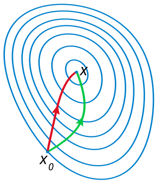
In calculus, Newton's method is an iterative method for finding the roots of a differentiable function , which are solutions to the equation . However, to optimize a twice-differentiable , our goal is to find the roots of . We can therefore use Newton's method on its derivative to find solutions to , also known as the critical points of . These solutions may be minima, maxima, or saddle points; see section "Several variables" in Critical point (mathematics) and also section "Geometric interpretation" in this article. This is relevant in optimization, which aims to find (global) minima of the function .
In mathematics, matrix calculus is a specialized notation for doing multivariable calculus, especially over spaces of matrices. It collects the various partial derivatives of a single function with respect to many variables, and/or of a multivariate function with respect to a single variable, into vectors and matrices that can be treated as single entities. This greatly simplifies operations such as finding the maximum or minimum of a multivariate function and solving systems of differential equations. The notation used here is commonly used in statistics and engineering, while the tensor index notation is preferred in physics.
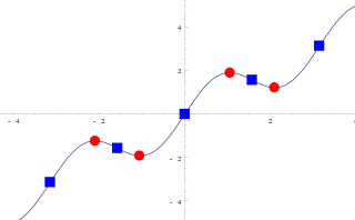
In mathematics, a critical point is the argument of a function where the function derivative is zero . The value of the function at a critical point is a critical value.
In mathematics, a change of variables is a basic technique used to simplify problems in which the original variables are replaced with functions of other variables. The intent is that when expressed in new variables, the problem may become simpler, or equivalent to a better understood problem.

In calculus, the second derivative, or the second-order derivative, of a function f is the derivative of the derivative of f. Informally, the second derivative can be phrased as "the rate of change of the rate of change"; for example, the second derivative of the position of an object with respect to time is the instantaneous acceleration of the object, or the rate at which the velocity of the object is changing with respect to time. In Leibniz notation: where a is acceleration, v is velocity, t is time, x is position, and d is the instantaneous "delta" or change. The last expression is the second derivative of position with respect to time.
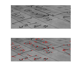
Corner detection is an approach used within computer vision systems to extract certain kinds of features and infer the contents of an image. Corner detection is frequently used in motion detection, image registration, video tracking, image mosaicing, panorama stitching, 3D reconstruction and object recognition. Corner detection overlaps with the topic of interest point detection.
In image processing, ridge detection is the attempt, via software, to locate ridges in an image, defined as curves whose points are local maxima of the function, akin to geographical ridges.
In differential calculus, there is no single uniform notation for differentiation. Instead, various notations for the derivative of a function or variable have been proposed by various mathematicians. The usefulness of each notation varies with the context, and it is sometimes advantageous to use more than one notation in a given context. The most common notations for differentiation are listed below.
The Hessian affine region detector is a feature detector used in the fields of computer vision and image analysis. Like other feature detectors, the Hessian affine detector is typically used as a preprocessing step to algorithms that rely on identifiable, characteristic interest points.
In mathematics, the method of steepest descent or saddle-point method is an extension of Laplace's method for approximating an integral, where one deforms a contour integral in the complex plane to pass near a stationary point, in roughly the direction of steepest descent or stationary phase. The saddle-point approximation is used with integrals in the complex plane, whereas Laplace’s method is used with real integrals.
In mathematical analysis and its applications, a function of several real variables or real multivariate function is a function with more than one argument, with all arguments being real variables. This concept extends the idea of a function of a real variable to several variables. The "input" variables take real values, while the "output", also called the "value of the function", may be real or complex. However, the study of the complex-valued functions may be easily reduced to the study of the real-valued functions, by considering the real and imaginary parts of the complex function; therefore, unless explicitly specified, only real-valued functions will be considered in this article.


